
Performance#
There are multiple parts in dynasor that can be computationally expensive, and depending on the use case different parts of the code can become performance limiting. The most time-consuming part of the dynamic structure factor calculations is usually the calculation of the Fourier transformed densities. This part is implemented in numba, and is significantly accelerated by parallelization. See below for run times of typical use cases.
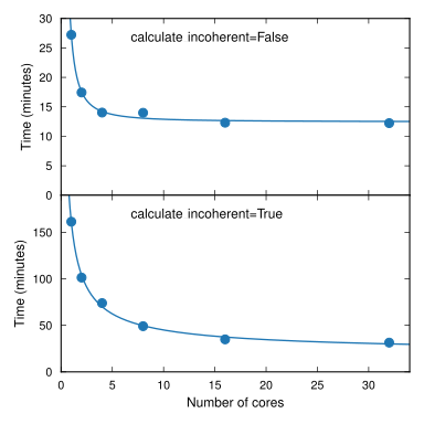
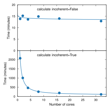
If trajectory reading and other overheads are disregarded and the incoherent part is not evaluated (calculate_incoherent=False), calculations should scale as N_qpts * N_atoms * max_frames.
Here N_qpts and N_atoms refer to the number of \(\boldsymbol{q}\)-points and atoms respectively.
Correlating the density between different frames in the window is often very fast and thus simulations often do not scale with time_window.
If the incoherent part (calculate_incoherent=True) is evaluated, calculations will typically scale as N_qpts * N_atoms * max_frames * time_window.
The dynasor calculations will typically become slower when calculating the incoherent intermediate scattering function.
Parallelization#
Parallelization is done over \(\boldsymbol{q}\)-points (N_qpts) when calculating the densities.
By default the calculations will be parallelized over all available cores.
Correlating the densities between frames is a cheap numpy operation and runs serially.
GPU backends#
The densities can also be evaluated on a CUDA GPU.
Call set_compute_config with backend='torch' or backend='cupy' before computing.
The kernel then runs about an order of magnitude faster than the numba kernel, while trajectory reading and the correlation step stay on the CPU and limit the gain for the calculation as a whole.
See the backends page for measured speedups, the precision and batch size settings, and the parts of a calculation that stay on the CPU.
Typical use cases#
Here we will consider a few typical use-cases in order to provide a rough estimate for how long typical calculations may take, and how calculations may scale with number of available cores.
Few \(\boldsymbol{q}\)-points#
Below are some time estimates for a three-component system of about 40,000 atoms and with a trajectory containing 10,000 snapshots. Here, only 5 high-symmetry \(\boldsymbol{q}\)-points are used as is typical when analyzing solids. The time window is set to 1000. Note that reading the trajectory (xyz format) accounts for a large part of the total computational time.
Many thousands of \(\boldsymbol{q}\)-points#
Below are some time estimates for a three-component system of about 10,000 atoms and with a trajectory containing 10,000 snapshots. Here, we consider 1000 \(\boldsymbol{q}\)-points and conduct a spherical average over \(\boldsymbol{q}\)-points. The time window is set to 400.
Trajectory reading#
The time spent on trajectory reading can be significant for plain-text formats (e.g., XYZ and LAMMPS dump). Therefore, if possible, we recommend using the binary formats if performance is essential and trajectory reading is a computational bottleneck. The benchmarks below were run on a normal modern desktop computer. Within each format the fastest reader comes first. MDAnalysis is the fastest reader for the binary GROMACS and NetCDF formats, OVITO for the plain-text formats.
Trajectory |
Reader |
N atoms |
Time |
|---|---|---|---|
Extended XYZ |
ovito |
20,480 |
40.51 s |
Extended XYZ |
internal |
20,480 |
1 min 14.4 s |
GROMACS TRR |
MDAnalysis |
42,464 |
49.22 s |
GROMACS XTC |
MDAnalysis |
42,464 |
11.30 s |
GROMACS XTC |
ovito |
42,464 |
26.93 s |
LAMMPS dump |
ovito |
16,384 |
33.83 s |
LAMMPS dump |
MDAnalysis |
16,384 |
4 min 53.1 s |
LAMMPS dump |
internal |
16,384 |
5 min 26.8 s |
NetCDF |
MDAnalysis |
20,480 |
8.45 s |
NetCDF |
ovito |
20,480 |
14.30 s |