Workflow

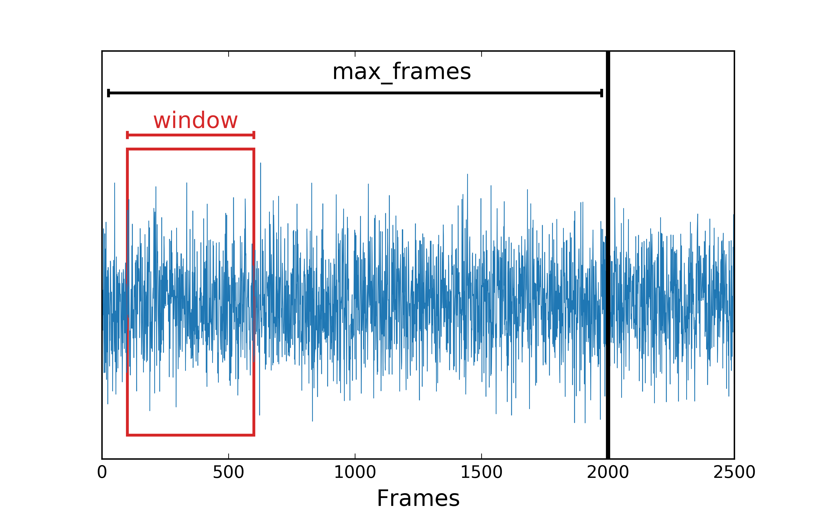
Schematic illustration of the workflow in dynasor. Text in red marks user inputs. The time window, indicated in blue, is moved through the trajectory until the specified maximum number of frames is reached.

Here, some additional information regarding the input parameters is provided, specifically for calculating dynamic and static structure factors. Additional details concerning these input parameters can be found in the documentation of the python interface.

Internal units

Internally dynasor uses units of Ångström (Å) for length and femtosecond (fs) for time. This means that all calculated correlation functions will be in terms of these units.

The trajectory

The MD trajectory must have a constant (not varying with time) simulation cell. Furthermore, when analyzing dynamic properties of systems the microcanonical (NVE) ensemble is usually preferred over the canonical ensemble (NVT), as thermostats influence the dynamics of the system.

In order to resolve certain frequencies, e.g., in \(S(q, \omega)\), you need to make sure the time between two consecutive snapshots complies with the Nyquist-Shannon sampling theorem.

It is important to specify the correct units in your trajectory to the trajectory reader of dynasor, such that they can be correctly converted to internal dynasor units.

Trajectory formats

dynasor can parse multiple different trajectory formats.

It has native support for parsing trajectories in lammps dump format [LAMMPS Molecular Dynamics Simulator, 2015].

Trajectories in extended xyz format can be read with the help of ase [Larsen et al., 2017]. Note that velocities are stored as arrays with the name vel as written by gpumd (https://gpumd.org/). The reader is multithreaded.

dynasor also interfaces with python package MDAnalysis, which allows users to parse a vast set of different trajectory formats.

Atomic types

If you want to calculate the correlation functions for each atom type (or different groupings of atoms) separately you need to provide the atomic_indices parameter in the form of a dictionary, for example,

atomic_indices['Cs'] = [0, 3, 6, 9]
atomic_indices['Br'] = [1, 2, 4, 5, 7, 8, 10, 11]

Alternativley, you can provide an index file (Gromacs ndx-style) to group atoms. For some trajectory formats, it is also possible to read the atomic_indices directly from the trajectory by setting it to 'read_from_trajectory'. If atomic_indices is left unspecified all atoms are assumed to be of the same species.

The molten sodium chloride example demonstrates the usage of an index file and how partial correlation functions can be analyzed. For example, in the case of a small system containing eight water molecules one could employ the following index file

[ Hydrogen ]
2 5 8 11 14 17 20 23
3 6 9 12 15 18 21 24
[ Oxygen ]
1 4 7 10 13 16 19 22

Here, the numbers following each tag ([...]) specify the atomic indices that belong to the respective species.

q-space sampling parameters

dynasor can either directly evaluate the correlation function at certain \(\boldsymbol{q}\)-points (typically desirable for solid or crystalline materials) or average the correlation functions over \(\boldsymbol{q}\)-points with similar length. The latter means constructing spherical average over \(\boldsymbol{q}\)-points which (often) requires thousands of \(\boldsymbol{q}\)-points to be sampled to get good statistics.

Note that \(\boldsymbol{q}\)-points in dynasor are not in reduced coordinates but given as Cartesian coordinates (in inverse Å) and should include the factor \(2\pi\).

Spherical q-point sampling and averaging

dynasor provides functionality to generate \(\boldsymbol{q}\)-points on a 3D grid with the spacing set by the simulation cell up to to the maximum radius set by q_max in units of \(2\pi/Å\). The resulting correlation functions can then be averaged over \(\boldsymbol{q}\)-points that fall into the same radial bin, where the parameter q_bins determines the number of radial bins.

The number of \(\boldsymbol{q}\)-points can grow very large using a 3D grid, and hence slow down calculations. The maximum number of \(\boldsymbol{q}\)-points to scan is specified by max_points, which allows one to set an approximate upper limit for the number of \(\boldsymbol{q}\)-points. If the number of \(\boldsymbol{q}\)-points on the grid exceeds max_points \(\boldsymbol{q}\)-points will be randomly removed in such a way that the number of \(\boldsymbol{q}\)-points inside each bin is roughly uniformly distributed.

Illustration of \(\boldsymbol{q}\)-points in 2D (blue) and their grouping into spherical (radial) bins, with 8 radial bins and about 1000 \(\boldsymbol{q}\)-points.

Time sampling parameters

The two main time sampling parameters are the number of time lags window_size and maximum number of frames frame_stop. The window size is only relevant for dynamic correlation functions but not for static ones. The maximum number of frames sets a limit on how many frames are read from the trajectory file. The window size is the longest time for which correlations are computed and is given in terms of the number of frames.

Additionally, you can specify frame_step to only use every frame_step-th snapshot in the trajectory. For example if frame_step=1 every snapshot will be used while for frame_step=2 every other snapshot is used. The window_step parameter controls how far the window is moved each time, with a default value of 1. A larger value may lead to the calculation running faster but also possibly less converged correlation functions. Note that if window_step is larger than the time window some snapshots in the trajectory will be skipped entirely.

To demonstrate how frame_step and window_step interact consider a trajectory with snapshots indexed from 1 to 100, and with window_size=5. The following snapshots will enter in the two first windows for which the correlation function is computed:

frame_step = 1
window_step = 1
  window 0 : snapshots [0, 1, 2, 3, 4]
  window 1 : snapshots [1, 2, 3, 4, 5]

frame_step = 2
window_step = 1
  window 0 : snapshots [0, 2, 4, 6, 8]
  window 1 : snapshots [2, 4, 6, 8, 10]

frame_step = 1
window_step = 2
  window 0 : snapshots [0, 1, 2, 3, 4]
  window 1 : snapshots [2, 3, 4, 5, 6]

frame_step = 2
window_step = 2
  window 0 : snapshots [0, 2, 4, 6, 8]
  window 1 : snapshots [4, 6, 8, 10, 12]

Lastly, it is required to set the time difference, dt, between two consecutive snapshots in the trajectory in femto seconds in order to get everything in the correct units. Note that you should not change dt when you change frame_step.

Schematic illustration of sliding time-window averaging over a trajectory.

Incoherent intermediate scattering function

The calculation of the incoherent part of the intermediate scattering function is turned off by default. It can be activated by setting calculate_incoherent to True when using the python interface and --calculate-incoherent when using the command line interface.

Post-processing

After the correlation functions have been calculated the results are stored as numpy array in the Sample object. There are multiple post-processing functions available, such as conducting spherical averages over \(\boldsymbol{q}\)-points and weighting with atomic form factors.

Limitations

Sometimes problems can occur due to known FFT features such as folding and aliasing. We have found the filon integration to work well for most applications, but sometimes it might be useful to apply FFT filters/windows to get a more smooth spectrum in the frequency domain.

The concept of \(\boldsymbol{q}\)-points becomes muddy if the simulation box is changing (which is the case, e.g., for NPT MD simulations). Differences in positions between two frames with different boxes are not uniquely defined. Therefore only constant volume MD trajectories are supported in dynasor.