Liquid and Solid Aluminium
In this first example aluminium will be studied. n EAM potential was used [Phys. Rev. B 59, 3393 (1999)] to describe both the solid and liquid phases. The melting point was found to be about 1000 K. The lattice parameters used for the NVT MD simulations were found running NPT and averaging the box length.
Liquid
First we look at alumnium above the melting point at 1400 K, i.e., as a liquid using a cell comprising 2048 atom. For liquids a spherically average over \(\boldsymbol{q}\) is desirable. To compute static properties such as \(S(q)\) no time correlation needs to be computed which reduces the computation time a lot.
In the figure the structure factor \(S(q)\) is shown.
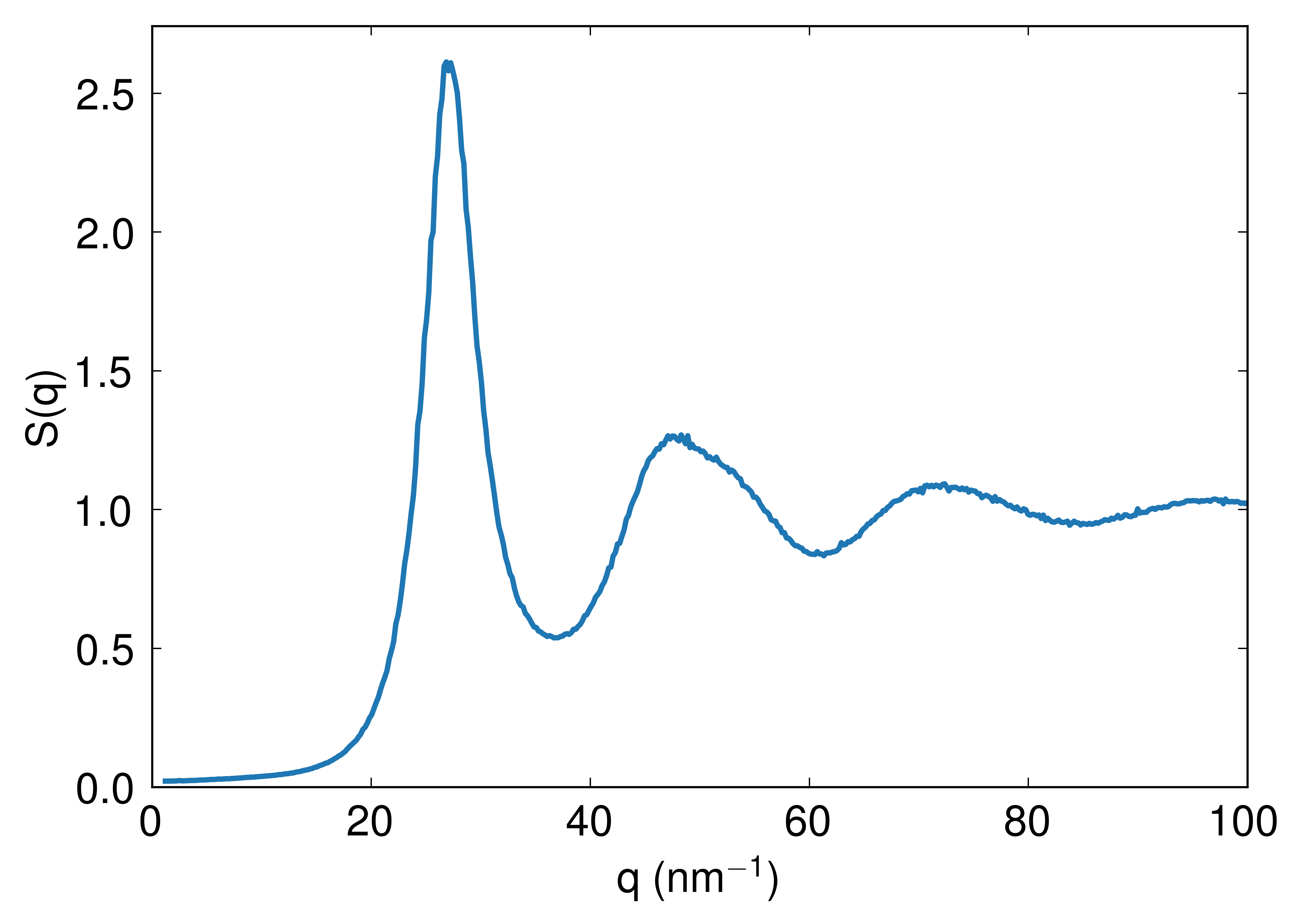
Structure factor \(S(q)\) computed by running run_dynasor_static.sh. The \(q=0\) point has been skipped for the structure factor due to \(S(0) = N\), see theory.
The structure factor is in good agreement with other MD simulations as well as with experimental data, see Figure 2 in [Mokshin and Yulemetyev, 2006].
A map of the dynamic structure factor and the two current correlations is seen below as a function of \(q\) and \(\omega\). The figure is cut at \(q=2.5~\text{nm}^{-1}\) because the resolution in \(\boldsymbol{q}\)-space is very poor below this point.
The intensity in \(C_l(q,\omega)\) is more pronounced than \(S(q,\omega)\), which means longitudinal vibrations are more easily observed in the current correlation rather than the dynamic structure factor.
These heatmaps seem to agree very well with spectral intensity plots in Figure 3 of [Mokshin and Yulemetyev, 2006]. The clear dispersion in \(C_l(q,\omega)\) agrees with the dispersion relation in Figure 4 of [Mokshin and Yulemetyev, 2006].
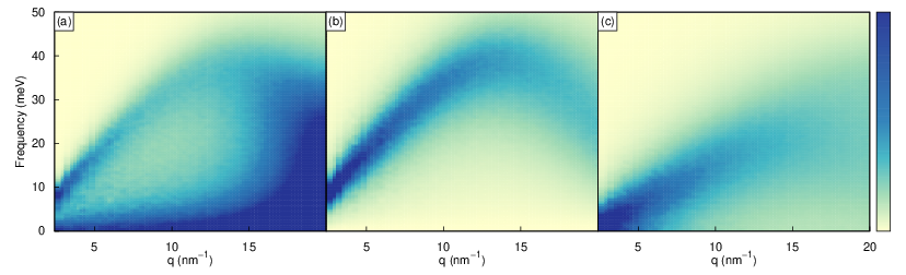
Dynamic structure factor (a), longitudinal current (b) and transverse current (c).
Crystalline
In this example we look at alumnium (FCC) below the melting point at \(T=300K\). Since the sampling along a path is much faster than doing a spherical average the number of atoms used here is 6912 (12x12x12 fcc).
The transverse and longitudinal current correlation is shown both in time and frequency for a single q-point. Fits to the analytical functions are also shown.
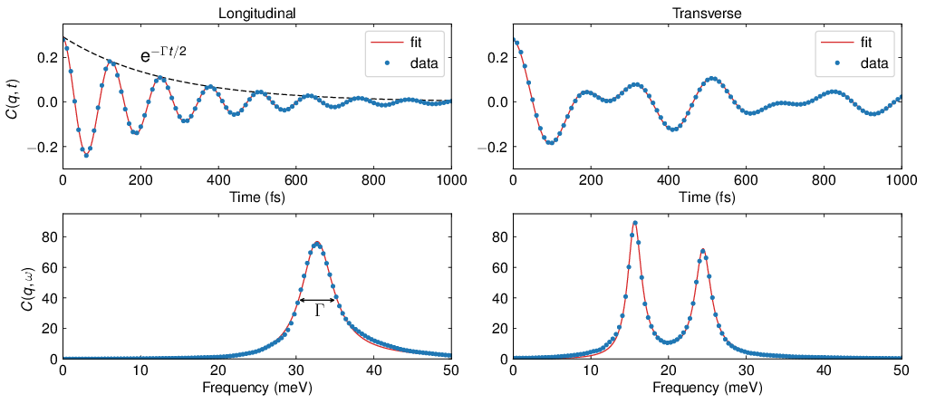
Longitudinal and transverse current correlations in both time and frequency.
Looking at the current correlations in time we see that the longitudinal is oscillating with one frequency and the transverse with two. This agrees with what is seen in the frequency domain.
The sum of the longitudinal and transverse current correlation is seen below together with the phonon dispersion calculated, using the same potential, by phonopy.
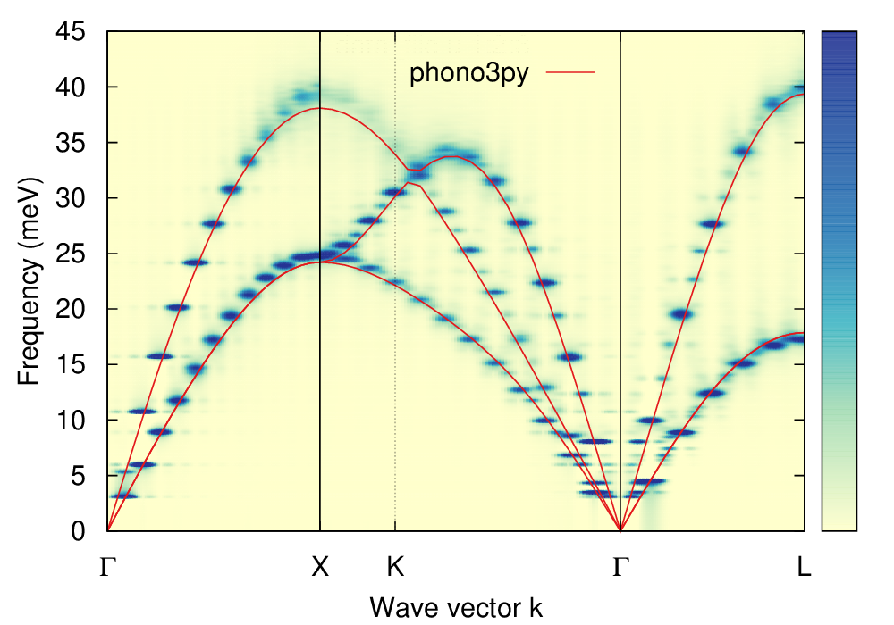
Sum of the longitudinal and transverse current heatmaps.
The agreement with the phonon dispersion calculated with phonopy is very good. The fact that there are discrete \(q\)-values that give rise to high intensitiy is due to the finite supercell size not supporting all kinds of oscillations.