Peak fitting

This tutorial demonstrates how one can analyze the current correlations and dynamic structure factor by fitting peaks to analytical expressions for a damped harmonic oscillators (DHO).

Damped harmonic oscillator

The details of the DHO model can be found in the theoretical background section. In short, the position autocorrelation function of a DHO is given by \begin{equation*} F(t) = A \mathrm{e}^{- t/\tau} \left ( \cos{ \omega_e t} + \frac{1}{\tau\omega_e}\sin{ \omega_e t}\right ), \end{equation*} where \(\omega_e = \sqrt{\omega_0^2 - 1/\tau^2}\) is the angular eigenfrequency of the DHO. The Fourier transform of the above is \begin{equation*} S(\omega) = A\frac{2\Gamma \omega_0^2}{(\omega^2 - \omega_0^2)^2 + (\Gamma\omega)^2}, \end{equation*} where \(\omega_0\) is the natural angular frequency, \(\Gamma\) the damping (lifetime \(\tau=2/\Gamma\)) and \(A\) an arbitrary amplitude of the DHO.

Note that for current correlations (and their respective Fourier transforms) one must use the velocity autocorrelation function for the DHO, whereas for the intermediate scattering function (and dynamic structure factor) the position autocorrelation function is used.

import numpy as np
import pandas as pd
from dynasor import read_sample_from_npz
from dynasor.units import radians_per_fs_to_meV
from matplotlib import pyplot as plt
from scipy.optimize import curve_fit

Al FCC

First, we will look at the current correlations, \(C_\text{L}(\boldsymbol{q}, t)\) and \(C_\text{T}(\boldsymbol{q}, t)\), in Al FCC at a temperature of T = 900 K and fit these with DHO models.

The full dispersion from current correlations is shown below, where blue corresponds to longitudinal modes and red to transverse modes.

Here, we will only consider fitting the current correlations for one q-point, namely \(\boldsymbol{q}=[0.5, 0.5, 0.0]\) which sits between K and \(\Gamma\).

This data is stored as a pandas dataframe in a csv file, obtained via sample.to_dataframe(q_index) (see here), and can be read using pandas.

# read data
alat = 4.05
df = pd.read_csv('Al_fcc_size24_T900_qindex38.csv')
display(df)

w = df.omega
t = df.time
Clqt = df.Clqt
Ctqt = df.Ctqt
Clqw = df.Clqw
Ctqw = df.Ctqw

	omega	time	Clqt	Clqt_X_X	Clqw	Clqw_X_X	Ctqt	Ctqt_X_X	Ctqw	Ctqw_X_X	Fqt_coh	Fqt_coh_X_X	Sqw_coh	Sqw_coh_X_X
0	0.000000	0	27.747023	27.747023	2.632250	2.632250	27.804061	27.804061	2.776075	2.776075	0.012116	0.012116	8.061254e-02	8.061254e-02
1	0.000157	5	26.699390	26.699390	3.549897	3.549897	27.373739	27.373739	34.885753	34.885753	0.011681	0.011681	1.425915e-01	1.425915e-01
2	0.000314	10	23.540678	23.540678	2.247025	2.247025	26.121036	26.121036	66.727080	66.727080	0.010453	0.010453	1.536352e-01	1.536352e-01
3	0.000471	15	18.562543	18.562543	3.889430	3.889430	24.101959	24.101959	48.080473	48.080473	0.008530	0.008530	8.122096e-02	8.122096e-02
4	0.000628	20	12.212002	12.212002	3.864050	3.864050	21.406585	21.406585	44.940541	44.940541	0.006063	0.006063	1.981069e-01	1.981069e-01
...	...	...	...	...	...	...	...	...	...	...	...	...	...	...
7996	1.256009	39980	-0.075647	-0.075647	-0.014731	-0.014731	0.051283	0.051283	-0.004358	-0.004358	0.000061	0.000061	3.456208e-06	3.456208e-06
7997	1.256166	39985	-0.062453	-0.062453	-0.012500	-0.012500	0.070549	0.070549	0.002383	0.002383	0.000052	0.000052	3.995259e-07	3.995259e-07
7998	1.256323	39990	-0.045894	-0.045894	-0.011104	-0.011104	0.086015	0.086015	0.005731	0.005731	0.000039	0.000039	3.718448e-06	3.718448e-06
7999	1.256480	39995	-0.024718	-0.024718	-0.004054	-0.004054	0.097392	0.097392	0.010066	0.010066	0.000022	0.000022	-2.560956e-06	-2.560956e-06
8000	1.256637	40000	0.001406	0.001406	-0.002088	-0.002088	0.105129	0.105129	-0.001084	-0.001084	0.000003	0.000003	-3.734499e-06	-3.734499e-06

8001 rows × 14 columns

First, we fit the data to a DHO in the time domain, although it could just as well be done in the frequency domain. The fitting can be accomplished in many ways, but here we simply use a least-square fit via SciPy’s curve_fit function. It is important to select some reasonable starting parameters in order to make the fit converge to a good solution. Note that while the fit is carried out in time domain, the resulting fit parameters (\(\omega_0, \Gamma, A\)) can directly be used in the frequency domain too.

from dynasor.tools.damped_harmonic_oscillator import acf_velocity_dho, psd_velocity_dho


# fitting longitudinal, in time domain
p0 = [30/radians_per_fs_to_meV, 2/radians_per_fs_to_meV, 1e4]  # initial guesses for parameters w0, Gamma, A
params_L, _ = curve_fit(acf_velocity_dho, t, Clqt, p0)

w0_L = params_L[0] * radians_per_fs_to_meV
gamma_L = params_L[1] * radians_per_fs_to_meV
print(f' Fitting results for C_L(q, t): w0 {w0_L:.2f} meV, gamma {gamma_L:.2f} meV')

# generate resulting dho data, in both time and frequency domain
t_lin = np.linspace(0, t.max(), 100000)
w_lin = np.linspace(0, w.max(), 100000)

Clqt_fit = acf_velocity_dho(t_lin, *params_L)
Clqw_fit = psd_velocity_dho(w_lin, *params_L)

 Fitting results for C_L(q, t): w0 35.00 meV, gamma 4.13 meV

Next, for fitting the tranvserse current correlation we need to employ a sum of two DHOs.

def two_acfs(t, w01, gamma1, A1, w02, gamma2, A2):
    acf1 = acf_velocity_dho(t, w01, gamma1, A1)
    acf2 = acf_velocity_dho(t, w02, gamma2, A2)
    return acf1 + acf2


def two_psds(t, w01, gamma1, A1, w02, gamma2, A2):
    psd1 = psd_velocity_dho(t, w01, gamma1, A1)
    psd2 = psd_velocity_dho(t, w02, gamma2, A2)
    return psd1 + psd2

# fitting transverse, in time domain
p0 = [15/radians_per_fs_to_meV, 2/radians_per_fs_to_meV, 1e4,
      30/radians_per_fs_to_meV, 2/radians_per_fs_to_meV, 1e4]
params_T, _ = curve_fit(two_acfs, t, Ctqt, p0)

w0_T1 = params_T[0] * radians_per_fs_to_meV
gamma_T1 = params_T[1] * radians_per_fs_to_meV
w0_T2 = params_T[3] * radians_per_fs_to_meV
gamma_T2 = params_T[4] * radians_per_fs_to_meV
print(f' Fitting results for C_T(q, t): w0 {w0_T1:.2f} meV, gamma {gamma_T1:.2f} meV and '
      f' w0 {w0_T2:.2f} meV, gamma {gamma_T2:.2f}')

# generate resulting dho data, in both time and frequency domain
t_lin = np.linspace(0, t.max(), 100000)
w_lin = np.linspace(0, w.max(), 100000)

Ctqt_fit = two_acfs(t_lin, *params_T)
Ctqw_fit = two_psds(w_lin, *params_T)

 Fitting results for C_T(q, t): w0 16.79 meV, gamma 1.83 meV and  w0 26.33 meV, gamma 1.78

Next, we plot the raw data and resulting fits.

fig, axes = plt.subplots(figsize=(5.8, 3.4), dpi=160, nrows=2, ncols=2, sharex='col', sharey='col')

# time domain
ax = axes[0][0]
kwargs_data = dict(ls='', marker='.', markersize=4, alpha=0.5)
ax.plot(t, Clqt, **kwargs_data)
kwargs_fit = dict(alpha=0.7)
ax.plot(t_lin, Clqt_fit, **kwargs_fit)
ax.plot(t_lin, Clqt[0] * np.exp(-t_lin * params_L[1]/2), '--k',
        alpha=0.8, lw=1, label=r'$\exp(-\Gamma t /2)$')
ax.set_ylabel(r'$C_\text{L}(\boldsymbol{q}, t)$')
ax.legend(frameon=False)

ax = axes[1][0]
ax.plot(t, Ctqt, **kwargs_data)
ax.plot(t_lin, Ctqt_fit, **kwargs_fit)
ax.set_ylabel(r'$C_\text{T}(\boldsymbol{q}, t)$')
ax.set_xlabel('Time (fs)')
ax.set_xlim(0, 1500)
#ax.set_ylim(-30, 30)

# frequency domain
ax = axes[0][1]
ax.plot(w * radians_per_fs_to_meV, Clqw, label='Data', **kwargs_data)
ax.plot(w_lin * radians_per_fs_to_meV, Clqw_fit, **kwargs_fit, label='Fit')
ax.set_ylabel(r'$C_\text{L}(\boldsymbol{q}, \omega)$')
ax.annotate('', xy=(w0_L - gamma_L/2 , Clqw_fit.max() / 2.0),
            xytext=(w0_L + gamma_L/2, Clqw_fit.max() / 2.0),
            arrowprops=dict(arrowstyle='<->'))
ax.text(w0_L, 0.6 * Clqw_fit.max()/2, r'$\Gamma$', ha='center')
ax.legend(frameon=False)

ax = axes[1][1]
ax.plot(w * radians_per_fs_to_meV, Ctqw, **kwargs_data)
ax.plot(w_lin * radians_per_fs_to_meV, Ctqw_fit, **kwargs_fit)
ax.set_ylabel(r'$C_\text{T}(\boldsymbol{q}, \omega)$')
ax.set_xlabel('Energy (meV)')
ax.set_xlim(10, 45)

fig.tight_layout()
fig.subplots_adjust(hspace=0)
fig.align_labels(axes)

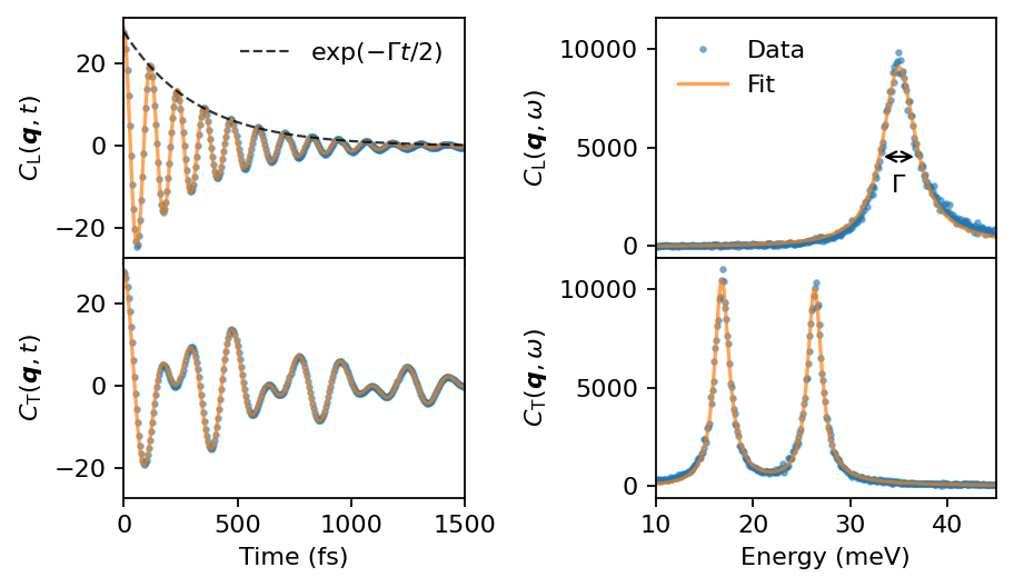
Note that, while the fits are carried out in the time domain, the corresponding DHO spectra match the data well in the frequency domain too. Generally, it is a good idea to plot the resulting fit in both the time and frequency domain, regardless of where the fit was performed, as a check of the procedure. In a simple system like this, is should not matter in which domain the fit is performed, but it might be easier to obtain a converged fit in one of the domains when more complex systems are considered.

Cubic BaZrO3

Additionally, we will consider a more anharmonic system, the cubic phase of BaZrO3 (BZO), with \(S(\boldsymbol{q}, \omega)\) data from this paper. We will analyze the low-frequency octahedral tilt phonon mode at the R-point (\(\boldsymbol{q}=[1.5, 0.5, 0.5]\)), at T = 300 K for three different pressure (0 GPa, 8 GPa, and 15.6 GPa). Note that this phonon mode is related to the phase transition between the cubic and tetragonal phases which occurs at around 16 GPa. The sample objects only contains \(S(\boldsymbol{q}, \omega)\) for this specific q-point.

Note that for overdamped modes the DHO is better represented using two timescales \(\tau_L\) and \(\tau_S\) instead of \(\omega_0\) and \(\Gamma\). These are defined as \begin{equation*} \tau_\text{S,L} = \frac{\tau}{1 \pm \sqrt{1-(\omega_0\tau)^2}}, \end{equation*} where \(\tau=2/\Gamma\).

# read data
P_vals =  [0.0, 8.0, 15.6]
data_dict = dict()
for P in P_vals:
    fname = f'BaZrO3_sample_T300_P{P:.1f}.npz'
    sample = read_sample_from_npz(fname)
    data_dict[P] = radians_per_fs_to_meV * sample.omega, sample.Sqw_coh[0]

Next, we visualize the three different spectra.

fig, ax = plt.subplots(1, 1, figsize=(3.4, 2.2), dpi=160)

for P, (w, Sqw) in data_dict.items():
    ax.plot(w, Sqw, '-', label=f'P={P} GPa', alpha=0.75)

ax.set_xlabel('Energy (meV)')
ax.set_ylabel(r'$S(\mathbf{q}, \omega)$')
ax.set_xlim(0, 20)
ax.set_ylim(1, 8000)
ax.set_yscale('log')
ax.legend(loc=1, frameon=False)

fig.tight_layout()

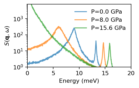
For 0 GPa we see two clear peaks at around 8 meV (octahedral tilt mode) and around 13 meV (acoustic Barium mode). Additionally, there exist multiple modes above 20 meV, but here we focus on the low frequency mode. For 15.6 GPa (close to the phase transition) one can clearly see that the tilt mode exhbits overdamped behaviour.

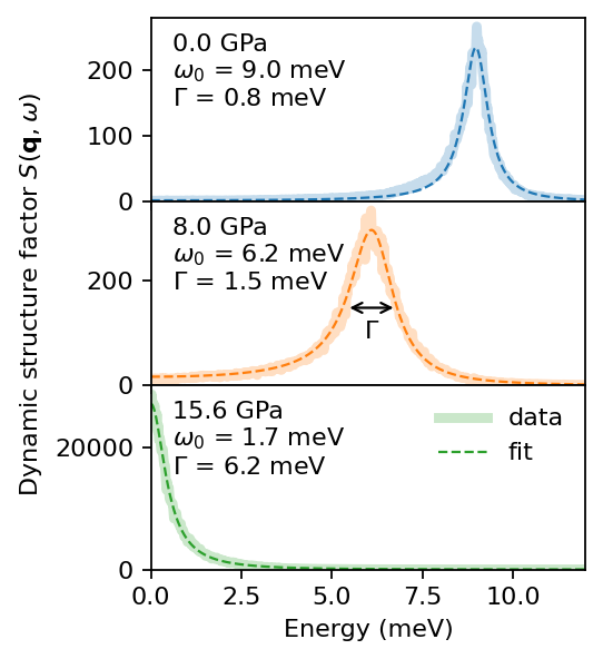
Next, we fit the corresponding spectra to DHOs, i.e., the fits are performed in the frequency domain.

Note that for 15.6 GPa we obtain \(\Gamma > 2 \omega_0\), meaning that the mode is overdamped.

from dynasor.tools.damped_harmonic_oscillator import psd_position_dho

fig, axes = plt.subplots(figsize=(3.4, 3.8), nrows=3, dpi=160, sharex=True)

colors_dict = dict()
colors_dict[0.0] = 'tab:blue'
colors_dict[8.0] = 'tab:orange'
colors_dict[15.6] = 'tab:green'

for ax, (P, (w, Sqw)) in zip(axes, data_dict.items()):

    # fit to DHO
    mask = w <= 12  # only use frequencies up to 12 meV
    p0 = [5.0, 2.0, 100]  # parameters guess
    params, _ = curve_fit(psd_position_dho, w[mask], Sqw[mask], p0=p0)
    w0, gamma, A = params
    print(f'{P:4.1f} GPa : w0= {w0:.2f} meV  gamma= {gamma:.2f} meV')

    ax.text(0.05, 0.82, f'{P:.1f} GPa', transform=ax.transAxes)
    ax.text(0.05, 0.67, rf'$\omega_0$ = {w0:.1f} meV', transform=ax.transAxes)
    ax.text(0.05, 0.52, rf'$\Gamma$ = {gamma:.1f} meV', transform=ax.transAxes)

    # plot
    w_lin = np.linspace(0, 12, 100000)
    S_fit = psd_position_dho(w_lin, *params)
    ax.plot(w, Sqw, '-', lw=4, alpha=0.25, color=colors_dict[P], label='data')
    ax.plot(w_lin, S_fit, '--', lw=1.0, color=colors_dict[P], label='fit')

    ax.set_xlim(0, 12)
    ax.set_ylim(bottom=0.0)

    # annotate roughly FWHM Gamma
    if P == 8.0:
        w_peak = np.sqrt(w0**2 - gamma**2 / 2.0)
        ax.annotate('', xy=(w_peak - gamma/2 , S_fit.max() / 2.0),
                    xytext=(w_peak + gamma/2, S_fit.max() / 2.0),
                    arrowprops=dict(arrowstyle='<->'))
        ax.text(w_peak, 0.6 * S_fit.max() / 2, r'$\Gamma$', ha='center')

axes[1].set_ylabel(r'Dynamic structure factor $S(\mathbf{q}, \omega)$')
axes[-1].set_xlabel('Energy (meV)')
axes[-1].legend(frameon=False)

fig.tight_layout()
fig.subplots_adjust(hspace=0)
fig.align_labels()

 0.0 GPa : w0= 8.99 meV  gamma= 0.82 meV
 8.0 GPa : w0= 6.18 meV  gamma= 1.48 meV
15.6 GPa : w0= 1.66 meV  gamma= 6.17 meV