Dynamic properties of FCC-Al#
This example demonstrates the analysis of the dynamics of crystalline aluminium in the face-centered cubic (FCC) structure via the dynamic structure factor as well as current correlation functions. Here, we use a rather small simulation cell (i.e., few q-points) and a short trajectory in order to make the tutorial run fast. In practice one needs to tune these parameters as well as the parameters used when calling dynasor for optimal results.
This example uses a trajectory that can be downloaded from Zenodo via
wget https://zenodo.org/records/10014454/files/dumpT300.NVT.atom.velocity.gz
or generated from scratch by running lammps using the input files provided.
[1]:
import numpy as np
import matplotlib.pyplot as plt
from ase import Atoms
from ase.build import bulk
from dynasor import compute_dynamic_structure_factors, Trajectory
from dynasor.qpoints import get_supercell_qpoints_along_path
from seekpath import get_path
Set up the trajectory#
dynasor supports multiple different trajectory formats via internal readers as well as via MDAnalysis and ASE. Here, we use the internal lammps reader.
[2]:
trajectory_filename = 'dumpT300.NVT.atom.velocity.gz'
traj = Trajectory(trajectory_filename,
                  trajectory_format='lammps_internal', frame_stop=10000)
INFO 2025-08-25 10:43:43: Assuming the trajectory has the default length unit (Ångström), since no unit was specified.
INFO 2025-08-25 10:43:43: Assuming the trajectory has the default time unit (fs), since no unit was specified.
INFO 2025-08-25 10:43:43: Trajectory file: dumpT300.NVT.atom.velocity.gz
INFO 2025-08-25 10:43:43: Total number of particles: 6912
INFO 2025-08-25 10:43:43: Number of atom types: 1
INFO 2025-08-25 10:43:43: Number of atoms of type X: 6912
INFO 2025-08-25 10:43:43: Simulation cell (in Angstrom):
[[48.78  0.    0.  ]
 [ 0.   48.78  0.  ]
 [ 0.    0.   48.78]]
A short summary of the content of the traj object can be obtained via the display (in notebooks) or print (in notebooks or scripts) command.
[3]:
display(traj)
Trajectory
| Field | Value | File name | dumpT300.NVT.atom.velocity.gz |
|---|---|
| Number of atoms | 6912 |
| Cell metric | [[48.78 0. 0. ] [ 0. 48.78 0. ] [ 0. 0. 48.78]] |
| Frame step | 1 |
| Atom types | ['X'] |
Set up path through Brillouin zone#
We now need to define the path through the Brillouin zone that we want to sample. The latter can be generated automatically for the crystal structure of interest using the seekpath package. To find the q-points along this path that can be sampled using the supercell used in the molecular dynamics simulations we use the function get_supercell_qpoints_along_path.
The primitive structure is generated using the bulk function from the ASE package.
[4]:
prim = bulk('Al', a=4.065)
path_info = get_path((
    prim.cell,
    prim.get_scaled_positions(),
    prim.numbers))
point_coordinates = path_info['point_coords']
path = path_info['path']
display(point_coordinates)
display(path)
{'GAMMA': [0.0, 0.0, 0.0],
 'X': [0.5, 0.0, 0.5],
 'L': [0.5, 0.5, 0.5],
 'W': [0.5, 0.25, 0.75],
 'W_2': [0.75, 0.25, 0.5],
 'K': [0.375, 0.375, 0.75],
 'U': [0.625, 0.25, 0.625]}
[('GAMMA', 'X'),
 ('X', 'U'),
 ('K', 'GAMMA'),
 ('GAMMA', 'L'),
 ('L', 'W'),
 ('W', 'X')]
[5]:
q_segments = get_supercell_qpoints_along_path(
    path, point_coordinates, prim.cell, traj.cell)
q_points = np.vstack(q_segments)
Run calculation of correlation functions#
We are now all set for calculating the dynamic structure factor as well as the current correlation functions, where the latter is triggered by setting calculate_currents=True. To obtain the correct units, the spacing between the frames (dt) must be specified in units of femtoseconds.
The following cell should take ten to twenty minutes to run on a common workstation.
Note: The Trajectory object is an “exhaustible iterable” , which means that once we have iterated over all frames, it is exhausted. Therefore, one needs to “reload” the trajectory before calling compute_dynamic_structure_factors again to ensure that the entire trajectory is available for analysis.
[6]:
%%time
sample = compute_dynamic_structure_factors(
    traj, q_points, dt=25.0, window_size=500,
    window_step=50, calculate_currents=True)
INFO 2025-08-25 10:43:45: Spacing between samples (frame_step): 1
INFO 2025-08-25 10:43:45: Time between consecutive frames in input trajectory (dt): 25.0 fs
INFO 2025-08-25 10:43:45: Time between consecutive frames used (dt * frame_step): 25.0 fs
INFO 2025-08-25 10:43:45: Time window size (dt * frame_step * window_size): 12500.0 fs
INFO 2025-08-25 10:43:45: Angular frequency resolution: dw = 0.000251 rad/fs = 0.165 meV
INFO 2025-08-25 10:43:45: Maximum angular frequency (dw * window_size): 0.125664 rad/fs = 82.713 meV
INFO 2025-08-25 10:43:45: Nyquist angular frequency (2pi / frame_step / dt / 2): 0.125664 rad/fs = 82.713 meV
INFO 2025-08-25 10:43:45: Calculating current (velocity) correlations
INFO 2025-08-25 10:43:45: Number of q-points: 48
INFO 2025-08-25 10:44:00: Processing window 0 to 500
INFO 2025-08-25 10:44:31: Processing window 1000 to 1500
INFO 2025-08-25 10:45:02: Processing window 2000 to 2500
INFO 2025-08-25 10:45:32: Processing window 3000 to 3500
INFO 2025-08-25 10:46:03: Processing window 4000 to 4500
INFO 2025-08-25 10:46:34: Processing window 5000 to 5500
INFO 2025-08-25 10:47:05: Processing window 6000 to 6500
INFO 2025-08-25 10:47:35: Processing window 7000 to 7500
INFO 2025-08-25 10:48:06: Processing window 8000 to 8500
INFO 2025-08-25 10:48:37: Processing window 9000 to 9500
CPU times: user 17min 57s, sys: 1.97 s, total: 17min 59s
Wall time: 5min 9s
As in the case of the trajectory, we can use the display or print commands to obtain a quick summary of the Sample object returned by the compute_dynamic_structure_factors function.
[7]:
display(sample)
DynamicSample
Simulation
| Name | Content |
|---|---|
| Angular frequency resolution | 0.0002513274122871834 |
| Atom types | ['X'] |
| Cell | [[48.78 0. 0. ] [ 0. 48.78 0. ] [ 0. 0. 48.78]] |
| Maximum time lag | 12500.0 |
| Number of frames | 10000 |
| Particle counts | {'X': 6912} |
| Time between frames | 25.0 |
Dimensions
| Field | Size |
|---|---|
| omega | (501,) |
| q_points | (48, 3) |
| time | (501,) |
History
| Function | Field | Content |
|---|---|---|
| compute_dynamic_structure_factors | dt | 25.0 |
| window_size | 500 | |
| window_step | 50 | |
| calculate_currents | True | |
| calculate_incoherent | False | |
| date_time | 2025-08-25T10:48:54 | |
| username | erhart | |
| hostname | pieweack | |
| dynasor_version | 2.2 |
To find out which correlation functions are included in a Sample object, one can inspect the available_correlation_functions property.
Tip: When working with an interactive Python interpreter, e.g., when using ipython or a jupyter instance, you can hit the <tab> key after writing sample. to show a list of possible completions.
[8]:
sample.available_correlation_functions
[8]:
['Clqt',
 'Clqt_X_X',
 'Clqw',
 'Clqw_X_X',
 'Ctqt',
 'Ctqt_X_X',
 'Ctqw',
 'Ctqw_X_X',
 'Fqt_coh',
 'Fqt_coh_X_X',
 'Sqw_coh',
 'Sqw_coh_X_X']
One can also write a Sample object to file and load it later for further processing. To write the object one should use the write_to_npz method.
[9]:
sample.write_to_npz('my_sample.npz')
The results can be read from file using the read_sample_from_npz function from the dynasor.sample module.
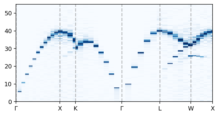
Visualize dynamic structure factor#
We can now visualize the dynamic structure factor \(S(\mathbf{q}, \omega)\), for example, in the form of a heatmap on the momentum-frequency plane.
In preparation, in the following cell we compute the running pairwise distance between q-points along the path.
[10]:
q_distances = []
q_labels = dict()

# starting point
qr = 0.0

# collect labels and q-distances along the entire q-point path
for it, q_segment in enumerate(q_segments):
    q_distances.append(qr)
    q_labels[qr] = path[it][0]
    for qi, qj in zip(q_segment[1:], q_segment[:-1]):
        qr += np.linalg.norm(qi - qj)
        q_distances.append(qr)

q_labels[qr] = path[-1][1]
q_distances = np.array(q_distances)
[11]:
from dynasor.units import radians_per_fs_to_meV as conversion_factor

fig = plt.figure(figsize=(5.2, 2.8), dpi=140)
ax = fig.add_subplot(111)
ax.pcolormesh(q_distances, conversion_factor * sample.omega,
              sample.Sqw_coh.T, cmap='Blues', vmin=0, vmax=4)

xticks = []
xticklabels = []
for q_dist, q_label in q_labels.items():
    ax.axvline(q_dist, c='0.5', alpha=0.5, ls='--')
    xticks.append(q_dist)
    xticklabels.append(q_label.replace('GAMMA', r'$\Gamma$'))

ax.set_xticks(xticks)
ax.set_xticklabels(xticklabels)

ax.set_xlim([0, q_distances.max()])
ax.set_ylim([0, 55])

ax.set_ylabel('Energy (meV)')

fig.tight_layout()
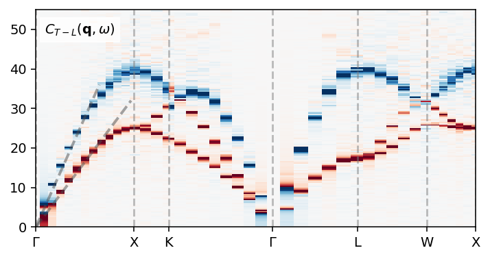
Visualize current correlations#
We can also plot the longitudinal and transverse current correlation heatmaps. In the longitudinal current correlation function one can observe the longitudinal branch that is also visible in the dynamic structure factor. Compared to the dynamic structure factor, the transverse current correlation function also reveals a transverse mode. The combination of the two (shown below) thus contains the full dispersion.
[12]:
fig = plt.figure(figsize=(5.2, 2.8), dpi=140)
ax = fig.add_subplot(111)
ax.pcolormesh(q_distances, conversion_factor * sample.omega,
              sample.Clqw.T - sample.Ctqw.T,
              cmap='RdBu', vmin=-6000, vmax=6000)

ax.plot([0, 1.0], [0, 36], alpha=0.5, ls='--', c='0.3', lw=2)
ax.plot([0, 1.5], [0, 32], alpha=0.5, ls='--', c='0.3', lw=2)

ax.text(0.02, 0.89, r'$C_{T-L}(\mathbf{q}, \omega)$', transform=ax.transAxes,
        bbox={'color': 'white', 'alpha': 0.8, 'pad': 3})

xticks = []
xticklabels = []
for q_dist, q_label in q_labels.items():
    ax.axvline(q_dist, c='0.5', alpha=0.5, ls='--')
    xticks.append(q_dist)
    xticklabels.append(q_label.replace('GAMMA', r'$\Gamma$'))

ax.set_xticks(xticks)
ax.set_xticklabels(xticklabels)

ax.set_xlim([0, q_distances.max()])
ax.set_ylim([0, 55])

ax.set_ylabel('Energy (meV)')

fig.tight_layout()