Mode projection#
In this tutorial we demonstrate how to use dynasor to study the dynamics of phonon modes. We will explore the ModeProjector object, which can be used together with force constants to obtain information about the dynamics in the system based on the harmonic approximation. The projector maps between real space atomic displacements u and inverse lattice phonon coordinates Q.
First, we construct the non-cubic primitive cell and cubic supercell using ase
[1]:
from ase.build import bulk

prim = bulk('Al', cubic=False)
repeat = 2
unit = bulk('Al', cubic=True)
supercell = unit.repeat(repeat)
Next, we need to set up phonopy and for that we need the repetition matrix P connecting the cell of the primitive structure to the supercell. This matrix can be found using a utility function in dynasor. Be careful, however, because phonopy requires the transpose of this matrix.
[2]:
from dynasor.tools.structures import get_P_matrix

P_matrix = get_P_matrix(prim.cell, supercell.cell)

print(P_matrix)
[[-2  2  2]
 [ 2 -2  2]
 [ 2  2 -2]]
Now we are ready to create the phonopy object and generate displaced supercells to create the force constant matrix. We use the built in emt calculator from ase for simplicity and utility functions from calorine.
[3]:
from calorine.tools.phonons import phonopy_to_ase, get_force_constants
from phonopy import Phonopy
from ase.calculators.emt import EMT

phonon = get_force_constants(prim, EMT(), supercell_matrix=P_matrix.T)
fc2_phonopy = phonon.force_constants
The internal phonopy supercell object is permuted relative to our original supercell. Either the supercell of phonopy can be used for subsequent calculations or the force constants need to be permuted. For this there is again a utility function in dynasor
[4]:
from dynasor.tools.structures import find_permutation

supercell_phonopy = phonopy_to_ase(phonon.supercell)

p = find_permutation(supercell_phonopy, supercell)

fc2 = fc2_phonopy[p][:,p]
We are now ready with the setup and can construct the ModeProjector
[5]:
from dynasor import ModeProjector

mp = ModeProjector(prim, supercell, fc2)

print(mp)
### ModeProjector ###
Supercell:
Number of atoms:      32
Volume:               531.441
Number of unit cells: 32
Cell:
[[8.1                 , 0.0                 , 0.0                 ],
 [0.0                 , 8.1                 , 0.0                 ],
 [0.0                 , 0.0                 , 8.1                 ]]
P-matrix:
[[-2                  , 2                   , 2                   ],
 [2                   , -2                  , 2                   ],
 [2                   , 2                   , -2                  ]]
Primitive cell:
Number of atoms:        1
Volume:                 16.608
Atomic species present: {'Al'}
Atomic numbers present: {13}
Cell:
[[0.0                 , 2.025               , 2.025               ],
 [2.025               , 0.0                 , 2.025               ],
 [2.025               , 2.025               , 0.0                 ]]

Ind  Sym  Num  Mass (Da) x         y         z         a         b         c
0    Al   13   26.98     0.000     0.000     0.000     0.000     0.000     0.000
                                 +


                                     +              +  +          + +


                                                                               +
                                                   +


+


-++++++++++++++++++++++++++++++++-+++-+++++++++++++--++-++++++++++-+-++++++++++-
|-0.00      THz                                                            7.99|
Printing the ModeProjector reveals some basic information about the primitive and supercell as well as an ASCII representation of the density of states. Under the hood the dynamical matrix has been constructed and diagonalized at each commensurate lattice point. The information about which q-points are supported is available in the reduced and cartesian arrays. Let’s print the first three points.
[6]:
for index, qp in enumerate(mp.q_reduced[:3]):
    print(f'{index:<5}{qp}')
0    [0. 0. 0.]
1    [0.  0.  0.5]
2    [0.   0.25 0.25]
From the above, we can note that the q-points are stored as reduced coordinates relative to the inverse primitive cell. Information about the primitive and supercell can be accessed by primitive and supercell respectively.
[7]:
print(mp.primitive)
Primitive cell:
Number of atoms:        1
Volume:                 16.608
Atomic species present: {'Al'}
Atomic numbers present: {13}
Cell:
[[0.0                 , 2.025               , 2.025               ],
 [2.025               , 0.0                 , 2.025               ],
 [2.025               , 2.025               , 0.0                 ]]

Ind  Sym  Num  Mass (Da) x         y         z         a         b         c
0    Al   13   26.98     0.000     0.000     0.000     0.000     0.000     0.000
[8]:
print(mp.supercell)
Supercell:
Number of atoms:      32
Volume:               531.441
Number of unit cells: 32
Cell:
[[8.1                 , 0.0                 , 0.0                 ],
 [0.0                 , 8.1                 , 0.0                 ],
 [0.0                 , 0.0                 , 8.1                 ]]
P-matrix:
[[-2                  , 2                   , 2                   ],
 [2                   , -2                  , 2                   ],
 [2                   , 2                   , -2                  ]]
Primitive cell:
Number of atoms:        1
Volume:                 16.608
Atomic species present: {'Al'}
Atomic numbers present: {13}
Cell:
[[0.0                 , 2.025               , 2.025               ],
 [2.025               , 0.0                 , 2.025               ],
 [2.025               , 2.025               , 0.0                 ]]

Ind  Sym  Num  Mass (Da) x         y         z         a         b         c
0    Al   13   26.98     0.000     0.000     0.000     0.000     0.000     0.000
In particular, the Cartesian q-vector can be constructed by
[9]:
import numpy as np

for index, q in enumerate(mp.q_reduced[:3]):
    q_cart = q @ (2*np.pi*mp.primitive.inv_cell)
    print(index, q, q_cart)
0 [0. 0. 0.] [0. 0. 0.]
1 [0.  0.  0.5] [ 0.77570189  0.77570189 -0.77570189]
2 [0.   0.25 0.25] [0.77570189 0.         0.        ]
For convenience these can also be accessed through
[10]:
print(mp.q_cartesian[:3])
[[ 0.00000000e+00  0.00000000e+00  0.00000000e+00]
 [ 7.75701890e-01  7.75701890e-01 -7.75701890e-01]
 [ 7.75701890e-01  2.27536266e-17 -2.27536266e-17]]
In addition, q-points can also be accessed by index from the ModeProjector, or by call providing the reduced q-vector.
[11]:
qp_1 = mp[1]
qp_2 = mp((0, 1/4, 1/4))

print(qp_1)
print(qp_2)
### q-point ###
Index:       1
Reduced:     [0.  0.  0.5]
Cartesian:   [0.78, 0.78, -0.78] rad/Å
Wavenumber:  1.34 rad/Å
Wavelength:  4.68 Å
q-minus:     1 [0.  0.  0.5]
Real:        True
Omegas:      [3.30, 3.30, 7.92] THz
### q-point ###
Index:       2
Reduced:     [0.   0.25 0.25]
Cartesian:   [0.78, 0.00, -0.00] rad/Å
Wavenumber:  0.78 rad/Å
Wavelength:  8.10 Å
q-minus:     7 [0.   0.75 0.75]
Real:        False
Omegas:      [3.78, 3.78, 5.18] THz
Printing the q-point reveals more detailed information. Notice that (0, 1/4, 1/4) is not real since its counterpropagating wave exists at another point in our supercell. This means that the amplitudes of these two modes are not independent. To access the q-point of the counterpropagating wave we can simply do
[12]:
print(qp_2.q_minus)
### q-point ###
Index:       7
Reduced:     [0.   0.75 0.75]
Cartesian:   [2.33, -0.00, 0.00] rad/Å
Wavenumber:  2.33 rad/Å
Wavelength:  2.70 Å
q-minus:     2 [0.   0.25 0.25]
Real:        False
Omegas:      [3.78, 3.78, 5.18] THz
or
[13]:
print(mp(-qp_2.q_reduced))
### q-point ###
Index:       7
Reduced:     [0.   0.75 0.75]
Cartesian:   [2.33, -0.00, 0.00] rad/Å
Wavenumber:  2.33 rad/Å
Wavelength:  2.70 Å
q-minus:     2 [0.   0.25 0.25]
Real:        False
Omegas:      [3.78, 3.78, 5.18] THz
This information is also contained in the q_minus array of the ModeProjector
[14]:
assert mp.q_minus[qp_2.index] == qp_2.q_minus.index
From the q-point we can access detailed information about each band by indexing the q-point object.
[15]:
band_2 = qp_1[2]
print(band_2)
### Band ###
Band index:     2
q-point:        [1] [0.  0.  0.5]
Frequency:      7.92 THz
Polarization:
0.58-0.00j          0.58-0.00j          -0.58-0.00j
              Q                   P                   F
Value:        0.00+0.00j          0.00+0.00j          0.00+0.00j
Amplitude:    0.00                0.00                0.00
Phase:        0.00                0.00                0.00
Energy:       0.00                0.00                -0.00+0.00j
As expected from a zone boundary mode the polarization vector is purely real. The polarization W can be accessed from both the ModeProjector itself or from the QPoint as well as the Band objects.
[16]:
print(mp.polarizations[band_2.qpoint.index, band_2.index])
print(qp_1.polarizations[band_2.index])
print(band_2.polarization)
[[ 0.57735027-0.j  0.57735027-0.j -0.57735027-0.j]]
[[ 0.57735027-0.j  0.57735027-0.j -0.57735027-0.j]]
[[ 0.57735027-0.j  0.57735027-0.j -0.57735027-0.j]]
By printing the band we also see information about the current values of the amplitude (Q) and momentum (P) of the mode, as well as the force (F) acting on the mode. All of these properties can be accessed from the ModeProjector, QPoint and Band objects.
It is also possible to modify the mode amplitudes directly. The Q, P and F coordinates can be accessed by, e.g.,
[17]:
print(band_2.Q)
### Mode coordinate Q ###
band:      [2] 7.92 THz
q-point:   [1] [0.  0.  0.5]
Value:     0.00+0.00j Å√dmu
Amplitude: 0.00 Å√dmu
Phase:     0.00 radians
As a final exercise, let’s map out the 0K energy landscape for the current band and compare with the harmonic approximation. The mode amplitudes should follow a normal distribution with deviation \(k_BT/\omega^2\)
[18]:
from ase.units import kB
import numpy as np
max_amp = 1 * (kB * 300 / np.abs(band_2.omega)**2)
amplitudes = np.linspace(-max_amp, max_amp)

harmonic_energies = []
emt_energies = []

ideal = mp.supercell.to_ase()
ideal.calc = EMT()
E0 = ideal.get_potential_energy()

mp.set_Q(0)

for amp in amplitudes:
    band_2.Q.amplitude = amp
    atoms = mp.get_atoms()
    atoms.calc = EMT()

    harmonic_energies.append(mp.potential_energies.sum())
    emt_energies.append(atoms.get_potential_energy()- E0)
[19]:
from matplotlib import pyplot as plt

fig, ax = plt.subplots()

ax.plot(amplitudes, emt_energies, label='EMT energy')
ax.plot(amplitudes, harmonic_energies, ls='--', label='Harmonic energy')

ax.set_ylabel('Energy (eV)')
ax.set_xlabel('Mode amplitude (Å√Da)')

ax.legend()

fig.tight_layout()
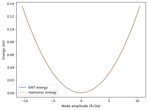
As demonstrated the harmonic approximation works well for aluminium for this mode.
There are many more functions and properties accessible via the ModeProjector, QPoint, Band and ComplexCoordinate objects respectively. You can consult the corresponding documentation pages for more information.