Weighting with form factors#
In this tutorial we demonstrate the weighting of structure factors with neutron scattering lengths and X-ray form factors, as different features in the full dispersion are visible depending on which probe is used in a scattering experiment. As a specific example we consider B2-ordered NiAl.
Because we return to the same system used in the multi-component tutorial, we assume that the molecular dynamics trajectories have already been prepared beforehand with GPUMD using the UNEP model as part of the “Dynamic properties of NiAl alloy” tutorial.
[1]:
import numpy as np
from ase.build import bulk
from ase.io import read
from matplotlib import pyplot as plt
from seekpath import get_path

from dynasor import compute_dynamic_structure_factors, Trajectory
from dynasor.qpoints import get_supercell_qpoints_along_path
from dynasor.units import radians_per_fs_to_meV
from dynasor.post_processing import \
    NeutronScatteringLengths, Weights, XRayFormFactors, get_weighted_sample
Compute correlation functions#
Here we set up the Trajectory, \(\boldsymbol{q}\)-points, and compute the dynamic structure factor. See the “Dynamic properties of NiAl alloy” tutorial for a more detailed description of these steps.
[2]:
# Set up trajectory
structure = read('model-ordered.xyz')
atomic_indices = {s: [a.index for a in structure if a.symbol == s]
                  for s in set(structure.symbols)}
traj = Trajectory('trajectory-ordered.nc',
                  trajectory_format='nc',
                  atomic_indices=atomic_indices,
                  length_unit='Angstrom',
                  time_unit='fs',
                  frame_step=1,
                  frame_stop=None)

# Set up path through Brillouin zone
repeats = 24  # We simulated a 24x24x24 supercell
prim = bulk('Al', a=traj.cell[0][0]/repeats)
path_info = get_path((prim.cell, prim.get_scaled_positions(), prim.numbers))
point_coordinates = path_info['point_coords']
path = path_info['path']

q_segments = get_supercell_qpoints_along_path(
    path, point_coordinates, prim.cell, traj.cell)
q_points = np.vstack(q_segments)
INFO 2025-08-25 11:11:50: Trajectory file: trajectory-ordered.nc
INFO 2025-08-25 11:11:50: Total number of particles: 27648
INFO 2025-08-25 11:11:50: Number of atom types: 2
INFO 2025-08-25 11:11:50: Number of atoms of type Ni: 13824
INFO 2025-08-25 11:11:50: Number of atoms of type Al: 13824
INFO 2025-08-25 11:11:50: Simulation cell (in Angstrom):
[[68.64  0.    0.  ]
 [ 0.   68.64  0.  ]
 [ 0.    0.   68.64]]
[3]:
%%time

# Compute correlation functions
delta_t = 5.0  # MD time step used (fs)
dump_every = 5  # How often the frames were dumped during MD

sample_raw = compute_dynamic_structure_factors(traj, q_points,
                                               dt=delta_t*dump_every,
                                               window_size=2000,
                                               window_step=100)
sample_raw.omega *= radians_per_fs_to_meV
display(sample_raw)
INFO 2025-08-25 11:12:02: Spacing between samples (frame_step): 1
INFO 2025-08-25 11:12:02: Time between consecutive frames in input trajectory (dt): 25.0 fs
INFO 2025-08-25 11:12:02: Time between consecutive frames used (dt * frame_step): 25.0 fs
INFO 2025-08-25 11:12:02: Time window size (dt * frame_step * window_size): 50000.0 fs
INFO 2025-08-25 11:12:02: Angular frequency resolution: dw = 0.000063 rad/fs = 0.041 meV
INFO 2025-08-25 11:12:02: Maximum angular frequency (dw * window_size): 0.125664 rad/fs = 82.713 meV
INFO 2025-08-25 11:12:02: Nyquist angular frequency (2pi / frame_step / dt / 2): 0.125664 rad/fs = 82.713 meV
INFO 2025-08-25 11:12:02: Number of q-points: 90
INFO 2025-08-25 11:12:19: Processing window 0 to 2000
INFO 2025-08-25 11:12:28: Processing window 1000 to 3000
INFO 2025-08-25 11:12:37: Processing window 2000 to 4000
INFO 2025-08-25 11:12:46: Processing window 3000 to 5000
INFO 2025-08-25 11:12:55: Processing window 4000 to 6000
INFO 2025-08-25 11:13:04: Processing window 5000 to 7000
INFO 2025-08-25 11:13:12: Processing window 6000 to 8000
INFO 2025-08-25 11:13:21: Processing window 7000 to 9000
INFO 2025-08-25 11:13:30: Processing window 8000 to 10000
INFO 2025-08-25 11:13:39: Processing window 9000 to 11000
INFO 2025-08-25 11:13:48: Processing window 10000 to 12000
INFO 2025-08-25 11:13:57: Processing window 11000 to 13000
INFO 2025-08-25 11:14:07: Processing window 12000 to 14000
INFO 2025-08-25 11:14:18: Processing window 13000 to 15000
INFO 2025-08-25 11:14:29: Processing window 14000 to 16000
INFO 2025-08-25 11:14:39: Processing window 15000 to 17000
INFO 2025-08-25 11:14:50: Processing window 16000 to 18000
INFO 2025-08-25 11:15:00: Processing window 17000 to 19000
INFO 2025-08-25 11:15:10: Processing window 18000 to 19999
INFO 2025-08-25 11:15:10: Processing window 19000 to 19999
DynamicSample
Simulation
| Name | Content |
|---|---|
| Angular frequency resolution | 6.283185307179586e-05 |
| Atom types | ['Al', 'Ni'] |
| Cell | [[68.64 0. 0. ] [ 0. 68.64 0. ] [ 0. 0. 68.64]] |
| Maximum time lag | 50000.0 |
| Number of frames | 20000 |
| Particle counts | {'Ni': 13824, 'Al': 13824} |
| Time between frames | 25.0 |
Dimensions
| Field | Size |
|---|---|
| omega | (2001,) |
| q_points | (90, 3) |
| time | (2001,) |
History
| Function | Field | Content |
|---|---|---|
| compute_dynamic_structure_factors | dt | 25.0 |
| window_size | 2000 | |
| window_step | 100 | |
| calculate_currents | False | |
| calculate_incoherent | False | |
| date_time | 2025-08-25T11:15:13 | |
| username | erhart | |
| hostname | pieweack | |
| dynasor_version | 2.2 |
CPU times: user 23min 44s, sys: 3.7 s, total: 23min 48s
Wall time: 3min 11s
Weighting with neutron scattering lengths#
To post-process the raw structure factor with weights of any kind, we need to first create a Weights object, which we then use to compute the weighted sample using the get_weighted_sample functionality.
We first illustrate how this is done in dynasor without bothering about the actual values of the scattering lengths, so we set the weights for both Ni and Al to 1. Instead of these dummy values, the weights could for example correspond to the charges, masses or, as we shall see below, scattering lengths or form factors, depending on the desired weighted correlation function.
[4]:
weights = Weights(dict(Ni=1, Al=1))
print(weights)
weights coherent:
  Ni: 1
  Al: 1
The weights we created like this are coherent weights. If we had computed the incoherent structure factor in compute_dynamic_structure_factors above (which is done using calculate_incoherent=True), we could have set the (generally different) incoherent scattering lengths as well, via a second dictionary:
[5]:
weights = Weights(dict(Ni=1, Al=1), weights_incoh=dict(Ni=1, Al=1))
print(weights)
weights coherent:
  Ni: 1
  Al: 1
weights incoherent:
  Ni: 1
  Al: 1
Now we want to generate some real weights, that we want to use to perform the weighting of the raw structure factor. This can be done manually by creating the Weights object as above, using your favorite table of neutron scattering lengths, but for convenience we provide tabulated values directly via NeutronScatteringLengths, taken from this NIST database, which in turn have been taken from Table 1 of Neutron News 3, 26
(1992); doi: 10.1080/10448639208218770.
[6]:
neutron_weights = NeutronScatteringLengths(['Ni', 'Al'])
print(neutron_weights)
weights coherent:
  Al: (3.449+0j)
  Ni: (10.331863+0j)
weights incoherent:
  Al: (0.256+0j)
  Ni: 0j
[7]:
sample_neutron = get_weighted_sample(sample_raw, neutron_weights)
display(sample_neutron)
DynamicSample
Simulation
| Name | Content |
|---|---|
| Angular frequency resolution | 6.283185307179586e-05 |
| Atom types | ['Al', 'Ni'] |
| Cell | [[68.64 0. 0. ] [ 0. 68.64 0. ] [ 0. 0. 68.64]] |
| Maximum time lag | 50000.0 |
| Number of frames | 20000 |
| Particle counts | {'Ni': 13824, 'Al': 13824} |
| Time between frames | 25.0 |
Dimensions
| Field | Size |
|---|---|
| omega | (2001,) |
| q_points | (90, 3) |
| time | (2001,) |
History
| Function | Field | Content |
|---|---|---|
| compute_dynamic_structure_factors | dt | 25.0 |
| window_size | 2000 | |
| window_step | 100 | |
| calculate_currents | False | |
| calculate_incoherent | False | |
| date_time | 2025-08-25T11:15:13 | |
| username | erhart | |
| hostname | pieweack | |
| dynasor_version | 2.2 | |
| get_weighted_sample | atom_type_map | None |
| weights_class | NeutronScatteringLengths | |
| weights_parameters | {'index': {0: 25, 1: 66, 2: 67, 3: 68, 4: 69, 5: 70}, 'species': {0: 'Al', 1: 'Ni', 2: 'Ni', 3: 'Ni', 4: 'Ni', 5: 'Ni'}, 'isotope': {0: 27, 1: 58, 2: 60, 3: 61, 4: 62, 5: 64}, 'abundance': {0: 1.0, 1: 0.6827, 2: 0.261, 3: 0.0113, 4: 0.0359, 5: 0.0091}, 'b_coh': {0: (3.449+0j), 1: (14.4+0j), 2: (2.8+0j), 3: (7.6+0j), 4: (-8.7+0j), 5: (-0.37+0j)}, 'b_inc': {0: (0.256+0j), 1: 0j, 2: 0j, 3: 0j, 4: 0j, 5: 0j}} | |
| date_time | 2025-08-25T11:15:13 | |
| username | erhart | |
| hostname | pieweack | |
| dynasor_version | 2.2 |
Visualize the neutron weighted structure factor#
We visualize the effect of the weighting by studying slices of \(S(\boldsymbol{q}, \omega)\) in \(\boldsymbol{q}\)-space. Note that we use to to_dataframe method of the Sample objects to obtain a pandas DataFrame, which provides some useful functionality, e.g., for data smoothing as shown below.
[8]:
fig, axes = plt.subplots(figsize=(7, 5.4), ncols=2, nrows=4, dpi=140, sharex=True)

qids = [48, 60]

for qid in qids:
    label = r'$\mathbf{q} =$'
    label += np.array_str(sample_raw.q_points[qid], precision=2, suppress_small=True)
    label += ' rad/Å'

    df = sample_raw.to_dataframe(qid)
    axes[0][0].plot(df.omega, df.Sqw_coh)
    axes[1][0].plot(df.omega, df.Sqw_coh_Al_Al)
    axes[2][0].plot(df.omega, df.Sqw_coh_Ni_Ni)
    axes[3][0].plot(df.omega, df.Sqw_coh_Al_Ni)

    df = sample_neutron.to_dataframe(qid)
    axes[0][1].plot(df.omega, df.Sqw_coh)
    axes[1][1].plot(df.omega, df.Sqw_coh_Al_Al)
    axes[2][1].plot(df.omega, df.Sqw_coh_Ni_Ni)
    axes[3][1].plot(df.omega, df.Sqw_coh_Al_Ni, label=label)

ax = axes[0][0]
ax.set_ylabel(r'$S(\omega)$')
ax.set_title('Raw')
ax.set_xlim(0, 60)

axes[1][0].set_ylabel(r'$S_{AlAl}(\omega)$')
axes[2][0].set_ylabel(r'$S_{NiNi}(\omega)$')
axes[3][0].set_ylabel(r'$S_{NiAl}(\omega)$')
axes[0][1].set_title('Neutron weighted')
axes[3][1].legend(fontsize='small')
for ax in axes[-1]:
    ax.set_xlabel('Energy (meV)')

fig.subplots_adjust(hspace=0, wspace=0.3)
fig.align_labels(axes)
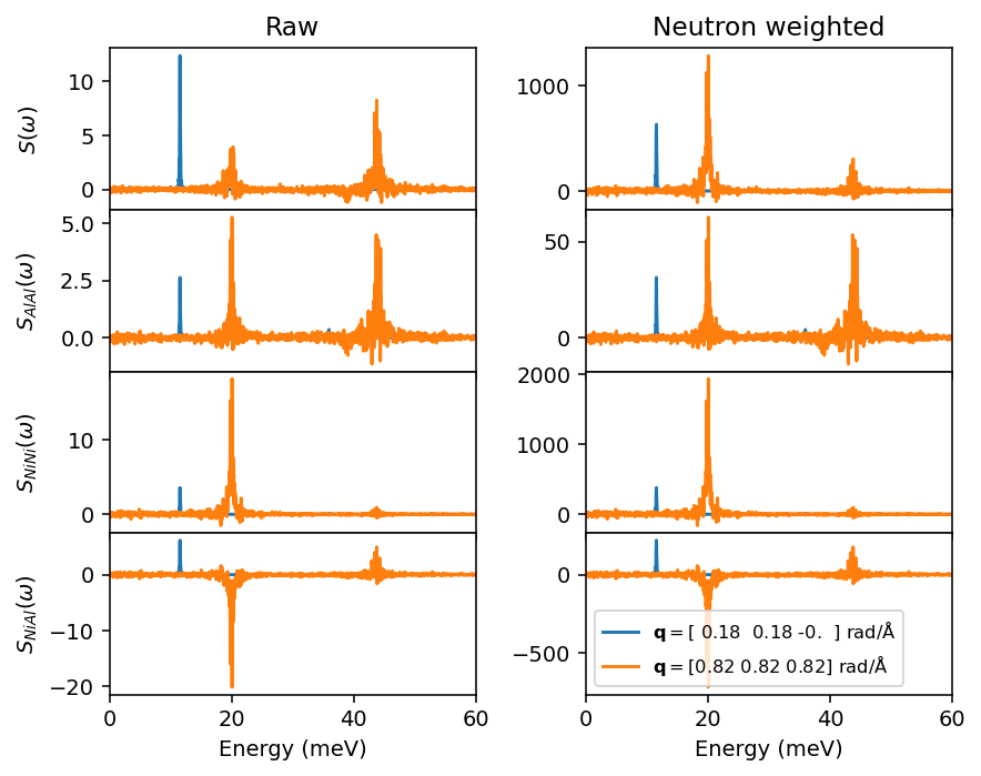
From the figures above, we can see that in each \(\boldsymbol{q}\)-slice of the raw total structure factor (top left), the low-frequency and the high-frequency peaks appear to be of similar height, while their intensities differ when the structure factor is weighted with neutron scattering lengths (top right). This is explained by the partial structure factors contributing in different amounts to the total, since the neutron scattering lengths for Ni and Al are different, so when adding the weighted partials up to obtain the total weighted structure factor the aspect ratio between the low-frequency and the high-frequency peaks changes compared to the raw total structure factor.
Weighting with X-ray form factors#
Now, we will do the same thing, but with X-ray form factors instead. Just as for the neutron weights, we provide tabulated values for X-ray form factors via XRayFormFactors. Here, there are two possible sources that can be specified, depending on the desired parametrization: source='waasmaier-1995' (taken from table 1 from D. Waasmaier, A. Kirfel, Acta Crystallographica Section A 51, 416 (1995); doi: 10.1107/S0108767394013292) or
source='itc-2006' (taken from Table 6.1.1.4. from International Tables for Crystallography, Volume C: Mathematical, physical, and chemical tables (2006)). If no source is specified, the default is waasmaier-1995. This is a convenience function, but if you would like to use a different source for the X-ray form factors, recall that it is possible to manually create a Weights object.
[9]:
xray_weights = XRayFormFactors(['Ni', 'Al'])
print(xray_weights)
weights coherent:
  Al: {'method': 'RHF', 'a1': 4.730796, 'b1': 3.620931, 'a2': 2.313951, 'b2': 43.051166, 'a3': 1.54198, 'b3': 0.09596, 'a4': 1.117564, 'b4': 100.932109, 'a5': 3.154754, 'b5': 1.555918, 'c': 0.139509}
  Ni: {'method': 'RHF', 'a1': 13.521865, 'b1': 4.077277, 'a2': 6.947285, 'b2': 0.286763, 'a3': 3.866028, 'b3': 14.622634, 'a4': 2.1359, 'b4': 71.966078, 'a5': 4.284731, 'b5': 0.004437, 'c': -2.762697}
While the neutron scattering lengths are independent of \(\boldsymbol{q}\), the X-ray form factors have a \(|\boldsymbol{q}|\)-dependence. For this reason, XRayFormFactors contains the parametrization, which allows for calculating the actual weight at the relevant \(\boldsymbol{q}\). Before performing the weighting, let’s visualize the q-dependence of the Ni and Al X-ray form factors.
[10]:
q_plot = np.linspace(0,6)
xray_ff_Ni_plot = [xray_weights.get_weight_coh('Ni', q) for q in q_plot]
xray_ff_Al_plot = [xray_weights.get_weight_coh('Al', q) for q in q_plot]

fig, ax = plt.subplots(figsize=(5, 3), ncols=1, nrows=1, dpi=140)
ax.plot(q_plot, xray_ff_Al_plot, label='Al', color='C3')
ax.plot(q_plot, xray_ff_Ni_plot, '--', label='Ni', color='C5')

ax.set_xlabel(r'$|\mathbf{q}|$ (rad/Å)')
ax.set_ylabel(r'$f(|\mathbf{q}|)$')
ax.legend()

fig.tight_layout()
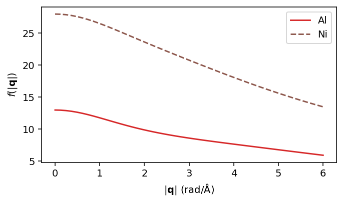
X-ray form factors roughly scale as the atomic number Z for different species, resulting in heavier elements being much more visible than lighter. This can be seen from the fact that Al (Z=13) and Ni (Z=28) differ by about a factor of two above.
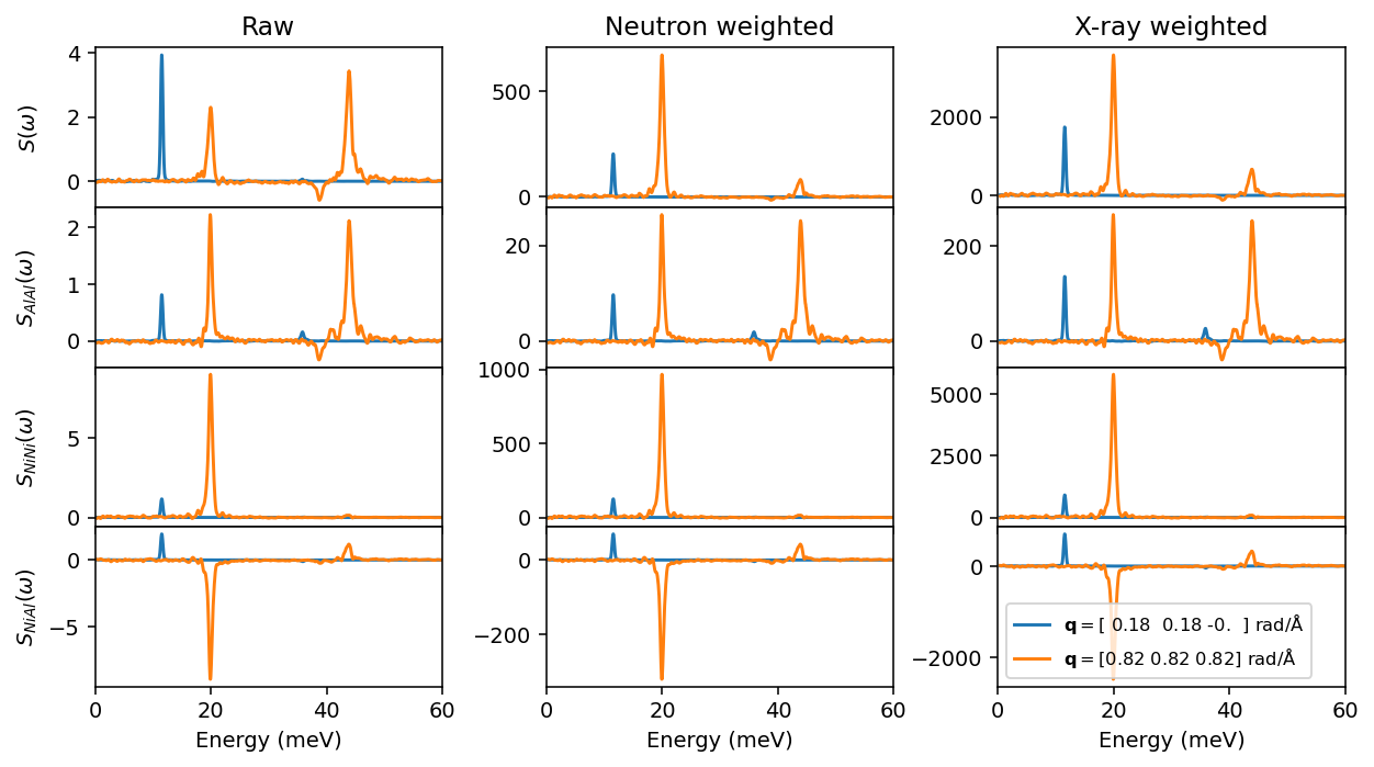
When actually using the XRayFormFactors to compute the weights, dynasor internally checks the \(\boldsymbol{q}\)-values for which the raw sample has been computed and calculates the X-ray form factor values at these \(\boldsymbol{q}\)-values, which means that computing the weighted sample is easily done in the same way as before:
[11]:
sample_xray = get_weighted_sample(sample_raw, xray_weights)
We can now compare the sample weighted with neutron scattering lengths to the sample weighted with the X-ray form factors. Again, we’ll look at some slices of \(S(\boldsymbol{q}, \omega)\) in \(\boldsymbol{q}\)-space.
[12]:
fig, axes = plt.subplots(figsize=(10.5, 5.4), ncols=3, nrows=4, dpi=140, sharex=True)

qids = [48, 60]

for qid in qids:
    label = r'$\mathbf{q} =$'
    label += np.array_str(sample_raw.q_points[qid], precision=2, suppress_small=True)
    label += ' rad/Å'

    df = sample_raw.to_dataframe(qid)
    axes[0][0].plot(df.omega, df.Sqw_coh)
    axes[1][0].plot(df.omega, df.Sqw_coh_Al_Al)
    axes[2][0].plot(df.omega, df.Sqw_coh_Ni_Ni)
    axes[3][0].plot(df.omega, df.Sqw_coh_Al_Ni)

    df = sample_neutron.to_dataframe(qid)
    axes[0][1].plot(df.omega, df.Sqw_coh)
    axes[1][1].plot(df.omega, df.Sqw_coh_Al_Al)
    axes[2][1].plot(df.omega, df.Sqw_coh_Ni_Ni)
    axes[3][1].plot(df.omega, df.Sqw_coh_Al_Ni)

    df = sample_xray.to_dataframe(qid)
    axes[0][2].plot(df.omega, df.Sqw_coh)
    axes[1][2].plot(df.omega, df.Sqw_coh_Al_Al)
    axes[2][2].plot(df.omega, df.Sqw_coh_Ni_Ni)
    axes[3][2].plot(df.omega, df.Sqw_coh_Al_Ni, label=label)

ax = axes[0][0]
ax.set_ylabel(r'$S(\omega)$')
ax.set_title('Raw')
ax.set_xlim(0, 60)

axes[1][0].set_ylabel(r'$S_{AlAl}(\omega)$')
axes[2][0].set_ylabel(r'$S_{NiNi}(\omega)$')
axes[3][0].set_ylabel(r'$S_{NiAl}(\omega)$')
axes[0][1].set_title('Neutron weighted')
axes[0][2].set_title('X-ray weighted')
axes[3][2].legend(fontsize='small')
for ax in axes[-1]:
    ax.set_xlabel('Energy (meV)')

fig.subplots_adjust(hspace=0, wspace=0.3)
fig.align_labels(axes)

The first thing to note is that the intensities of the total structure factor (first row) vary depending on the probe, which reflects the fact that the interaction strength between a probe and an atomic species varies depending on the probe.
Furthermore, it is possible to see the effect of the \(|\boldsymbol{q}|\)-dependence of the X-ray form factors in these figures. Take, for instance, the Al-Al partial structure factor (second row). When weighted with neutron scattering lengths, which do not depend on \(\boldsymbol{q}\), the ratio between the curves for the different \(\boldsymbol{q}\)-points does not change. For the X-ray form factors, however, we see that the low-frequency peak of the orange curve becomes higher than the low-frequency peak of the blue curve, opposite of the situation in the raw Al-Al partial structure factor, i.e., the ratio between the curves for different \(\boldsymbol{q}\)-points changes. This is an effect of the \(|\boldsymbol{q}|\)-dependence of the X-ray form factors. The orange curve is a slice at a \(\boldsymbol{q}\)-point with norm 0.26 rad/Å, while the blue curve is a slice at a \(\boldsymbol{q}\)-point with norm 1.43 rad/Å. As a result, the latter has a smaller X-ray form factor according to the previous plot that shows the \(|\boldsymbol{q}|\)-dependence of the X-ray form factors.
Smoothing data#
Finally, we demonstrate how one can easily smooth data using the rolling method of the DataFrame object. Here, we apply a Hamming window with a size of 20 along the energy axis. You can find more information about windowing operations in pandas on this page.
[13]:
fig, axes = plt.subplots(figsize=(10.5, 5.4), ncols=3, nrows=4, dpi=140, sharex=True)

qids = [48, 60]

for qid in qids:
    label = r'$\mathbf{q} =$'
    label += np.array_str(sample_raw.q_points[qid], precision=2, suppress_small=True)
    label += ' rad/Å'

    window = 20
    win_type = 'hamming'
    df = sample_raw.to_dataframe(qid)
    df = df.rolling(window=window, win_type=win_type).mean()
    axes[0][0].plot(df.omega, df.Sqw_coh)
    axes[1][0].plot(df.omega, df.Sqw_coh_Al_Al)
    axes[2][0].plot(df.omega, df.Sqw_coh_Ni_Ni)
    axes[3][0].plot(df.omega, df.Sqw_coh_Al_Ni)

    df = sample_neutron.to_dataframe(qid)
    df = df.rolling(window=window, win_type=win_type).mean()
    axes[0][1].plot(df.omega, df.Sqw_coh)
    axes[1][1].plot(df.omega, df.Sqw_coh_Al_Al)
    axes[2][1].plot(df.omega, df.Sqw_coh_Ni_Ni)
    axes[3][1].plot(df.omega, df.Sqw_coh_Al_Ni)

    df = sample_xray.to_dataframe(qid)
    df = df.rolling(window=window, win_type=win_type).mean()
    axes[0][2].plot(df.omega, df.Sqw_coh)
    axes[1][2].plot(df.omega, df.Sqw_coh_Al_Al)
    axes[2][2].plot(df.omega, df.Sqw_coh_Ni_Ni)
    axes[3][2].plot(df.omega, df.Sqw_coh_Al_Ni, label=label)

ax = axes[0][0]
ax.set_ylabel(r'$S(\omega)$')
ax.set_title('Raw')
ax.set_xlim(0, 60)

axes[1][0].set_ylabel(r'$S_{AlAl}(\omega)$')
axes[2][0].set_ylabel(r'$S_{NiNi}(\omega)$')
axes[3][0].set_ylabel(r'$S_{NiAl}(\omega)$')
axes[0][1].set_title('Neutron weighted')
axes[0][2].set_title('X-ray weighted')
axes[3][2].legend(fontsize='small')
for ax in axes[-1]:
    ax.set_xlabel('Energy (meV)')

fig.subplots_adjust(hspace=0, wspace=0.3)
fig.align_labels(axes)