Static structure factor in CsPbI3#
The static structure factor \(S(q)\), which is what is measured in diffraction experiments, is commonly used to identify and determine the crystal structure of a sample.
In this example we will analyze the static structure factor in the halide perovskite CsPbI3, which undergoes phase transitions from cubic (high temperature), to tetragonal (intermediate temperatures), and to orthorhombic (low temperatures).
Structure and potential files#
The relevant structure and potential files for carrying out this analysis can be found in this Zenodo repository. For example you can fetch these files via
wget https://zenodo.org/records/8014365/files/CsPbI3-CX-cubic-Pm-3m.xyz
wget https://zenodo.org/records/8014365/files/CsPbI3-CX-tetragonal-P4mbm.xyz
wget https://zenodo.org/records/8014365/files/nep-CsPbI3-CX.txt
MD simulations#
The MD simulations analyzed here are run with GPUMD and the nep-CsPbI3-CX.txt file mentioned above. The MD files (including the trajectories) can be fetched directly from Zenodo MD runs.
wget https://zenodo.org/records/10149723/files/md_runs.tar.gz
Afterwards they need to be unzipped and untarred, e.g., via
gunzip md_runs.tar.gz
tar xf md_runs.tar
[1]:
import numpy as np
import matplotlib.pyplot as plt
from ase.io import read, write
from dynasor.qpoints import get_spherical_qpoints
from dynasor import compute_static_structure_factors, Trajectory
from dynasor.post_processing import get_spherically_averaged_sample_smearing
\(S(\boldsymbol{q})\) for ideal structures#
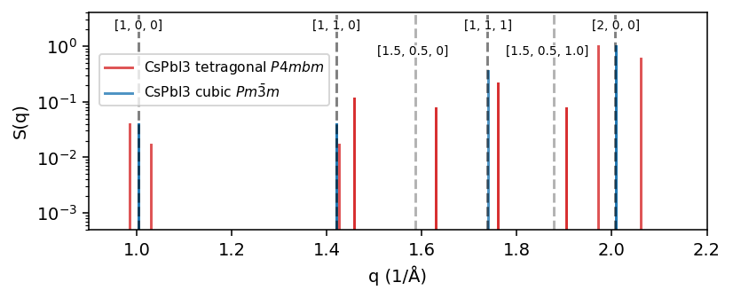
First we compute the structure factor, \(S(q)\), for the ideal CsPbI3 structures. Here, we normalize \(S(q)\) by number of atoms to more easily compare \(S(q)\) for structures with varying number of atoms.
For the cubic phase we expect peaks at the q-points \(\boldsymbol{q}=\frac{2\pi}{a}[i, j, k]\) for integer values of i, j, k. The cubic lattice parameter, \(a=6.26\) Å, is numerically quite close to \(2\pi\), meaning \(S(q)\) will exhibit peaks for the cubic phase at about \(q=1.0, \sqrt{2}, \sqrt{3}, 2.0\) \(Å^{-1}\) corresponding to \(\boldsymbol{q}=[1,0,0], [1, 1, 0], [1, 1, 1], [2, 0, 0]\).
In the tetragonal phase the x, y, z cubic symmetry is broken and z becomes distinct from x and y. This means that, e.g., the degenerate peaks \([1, 0, 0], [0, 1, 0], [0, 0, 1]\) in the cubic phase split into two peaks. Furthermore, since the tetragonal phase arises from a soft phonon mode instability at the M-point (\([0.5, 0.5, 0]\)), we expect additional peaks at e.g. \(q=1.58\) (\([1.5, 0.5, 0]\)) and \(q=1.87\) (\([1.5, 0.5, 1]\)).
To demonstrate this point we also mark these expected q-points in the figure below with dashed gray lines. Note that in order to get perfect agreement with the calculated \(S(q)\) of the real structure one would need to take into account the exact lattice parameters.
[2]:
structure_tags = ['CsPbI3-CX-tetragonal-P4mbm', 'CsPbI3-CX-cubic-Pm-3m']
data_dict = dict()
for structure_tag in structure_tags:

    # write dummy traj
    atoms = read(f'{structure_tag}.xyz')
    atoms.calc = None
    n_atoms = len(atoms)
    traj = [atoms for _ in range(2)]
    write('tmp_traj.xyz', traj)

    # setup traj
    traj = Trajectory('tmp_traj.xyz', trajectory_format='extxyz', atomic_indices='read_from_trajectory')

    # q-points
    q_max = 2.5
    q_points = get_spherical_qpoints(traj.cell, q_max=q_max)

    # compute Sq
    sample = compute_static_structure_factors(traj, q_points)
    q_norms = np.linalg.norm(sample.q_points, axis=1)
    data_dict[structure_tag] = q_norms, sample.Sq / n_atoms
INFO 2025-08-25 11:46:51: Assuming the trajectory has the default length unit (Ångström), since no unit was specified.
INFO 2025-08-25 11:46:51: Assuming the trajectory has the default time unit (fs), since no unit was specified.
INFO 2025-08-25 11:46:51: Trajectory file: tmp_traj.xyz
INFO 2025-08-25 11:46:51: Total number of particles: 10
INFO 2025-08-25 11:46:51: Number of atom types: 3
INFO 2025-08-25 11:46:51: Number of atoms of type Cs: 2
INFO 2025-08-25 11:46:51: Number of atoms of type I: 6
INFO 2025-08-25 11:46:51: Number of atoms of type Pb: 2
INFO 2025-08-25 11:46:51: Simulation cell (in Angstrom):
[[ 8.62193057e+00 -1.96501346e-14 -1.00257367e-15]
 [-9.98490387e-14  8.62193057e+00 -5.90070099e-16]
 [ 8.03089883e-16  4.00888754e-16  6.37484774e+00]]
INFO 2025-08-25 11:46:51: Number of q-points: 121
INFO 2025-08-25 11:46:52: Assuming the trajectory has the default length unit (Ångström), since no unit was specified.
INFO 2025-08-25 11:46:52: Assuming the trajectory has the default time unit (fs), since no unit was specified.
INFO 2025-08-25 11:46:52: Trajectory file: tmp_traj.xyz
INFO 2025-08-25 11:46:52: Total number of particles: 5
INFO 2025-08-25 11:46:52: Number of atom types: 3
INFO 2025-08-25 11:46:52: Number of atoms of type Cs: 1
INFO 2025-08-25 11:46:52: Number of atoms of type I: 3
INFO 2025-08-25 11:46:52: Number of atoms of type Pb: 1
INFO 2025-08-25 11:46:52: Simulation cell (in Angstrom):
[[ 6.25796103e+00 -2.33844250e-17 -2.53411308e-17]
 [-1.82080433e-17  6.25796103e+00  6.92635779e-16]
 [-8.47103199e-18  9.09518288e-17  6.25796103e+00]]
INFO 2025-08-25 11:46:52: Number of q-points: 81
[3]:
# plot setup
fig = plt.figure(figsize=(6.0, 2.5), dpi=140)
ax1 = fig.add_subplot()

colors = dict()
colors['CsPbI3-CX-tetragonal-P4mbm'] = 'tab:red'
colors['CsPbI3-CX-cubic-Pm-3m'] = 'tab:blue'

labels = dict()
labels['CsPbI3-CX-tetragonal-P4mbm'] = r'CsPbI$_3$ tetragonal $P4mbm$'
labels['CsPbI3-CX-cubic-Pm-3m'] = r'CsPbI$_3$ cubic $Pm\bar{3}m$'

xlim = [0.9, 2.2]
ylim = [0.0005, 4]
alpha = 0.8


# plot S(q) as vertical lines
for structure_tag, (q_norms, Sq) in data_dict.items():
    for q, S in zip(q_norms, Sq):
        ax1.plot([q, q], [0, S[0]], color=colors[structure_tag], alpha=alpha)
    ax1.plot(np.nan, np.nan, color=colors[structure_tag], alpha=alpha, label=labels[structure_tag])


# Mark the cubic gamma-points
alat = 6.26
alpha = 0.5
fs = 7
bbox = dict(facecolor='w', edgecolor='none', alpha=0.85, pad=0.0)

q_vecs = [[1, 0, 0], [1, 1, 0], [1, 1, 1], [2, 0, 0]]
for qvec in q_vecs:
    q = 2 * np.pi / alat * np.linalg.norm(qvec)
    ax1.axvline(x=q, ls='--', color='k', alpha=alpha)
    ax1.text(q -0.05, 0.5 * ylim[-1], str(qvec), fontsize=fs, bbox=bbox)

# Mark the cubic M-points
qvec_M1 = [1.5, 0.5, 0]
qvec_M2 = [1.5, 0.5, 1.0]
q_M1 = 2 * np.pi / alat * np.linalg.norm(qvec_M1)
q_M2 = 2 * np.pi / alat * np.linalg.norm(qvec_M2)
ax1.axvline(x=q_M1, ls='--', color='k', alpha=alpha-0.2)
ax1.axvline(x=q_M2, ls='--', color='k', alpha=alpha-0.2)
ax1.text(q_M1-0.08, 0.17 * ylim[-1], str(qvec_M1), fontsize=fs, bbox=bbox)
ax1.text(q_M2-0.1, 0.17 * ylim[-1], str(qvec_M2), fontsize=fs, bbox=bbox)


ax1.set_xlim(xlim)
ax1.set_ylim(ylim)
ax1.set_yscale('log')
ax1.legend(loc=1, fontsize=8, bbox_to_anchor=(0.4, 0.84))
ax1.set_xlabel('q (rad/Å)')
ax1.set_ylabel('S(q)')

fig.tight_layout()
\(S(\boldsymbol{q})\) from MD simulations#
When running MD simulations of larger supercells, the number of available q-points becomes large. Here, we can either sample selected q-points in specific regions of the BZ, see e.g. this paper.
Alternatively, we can sample all of the available q-points and e.g. conduct a spherical q-point average in order to mimic experimental powder diffraction data.
Spherical q-point average#
Spherical q-point averaging can be done in dynasor with the get_spherically_averaged_sample_... functions using either a binning method or Gaussian smearing method, here we use the latter meaning \begin{equation*}
S(q) = \sum_i w(\boldsymbol{q}_i, q) S(\boldsymbol{q}_i)
\end{equation*} where \(w(\boldsymbol{q}_i, q)\) is a Gaussian weight, i.e. \begin{equation*}
w(\boldsymbol{q}_i, q) \propto \exp{\left [ -\frac{1}{2} \left ( \frac{|\boldsymbol{q}_i| - q}{q_\text{width}} \right)^2 \right ]}
\end{equation*}
Below we compute and plot the raw \(S(q)\) and the Gaussian spherical averaged \(S(q)\) for one selected MD simulation to demonstrate it. One can play around with the width (standard deviation) of the Gaussian, q_width, in order to obtain a desirable looking structure factor.
Note: avoid choosing q_width much smaller than the spacing of q_norms (the q-grid you evaluate on). If it is, the smeared curve tends to become spiky and under-resolved.
[4]:
%%time

# parameters
q_max = 2.05
q_linspace = np.linspace(0, q_max, 1000)
q_width = 0.1

# setup traj
tag = f'tetra_size8_T450_nframes1000'
dirname = f'md_runs/NVT_{tag}/'
traj = Trajectory(dirname + 'movie.nc', trajectory_format='nc')

# generate all q-points in supercell
q_points = get_spherical_qpoints(traj.cell, q_max=q_max)

# sort q-points by length
argsort = np.argsort(np.linalg.norm(q_points, axis=1))
q_points = q_points[argsort]

# compute Sq
sample = compute_static_structure_factors(traj, q_points)
INFO 2025-08-25 11:46:52: Length unit Angstrom and time unit ps inferred from trajectory.
INFO 2025-08-25 11:46:52: Trajectory file: md_runs/NVT_tetra_size8_T450_nframes1000/movie.nc
INFO 2025-08-25 11:46:52: Total number of particles: 5120
INFO 2025-08-25 11:46:52: Number of atom types: 1
INFO 2025-08-25 11:46:52: Number of atoms of type X: 5120
INFO 2025-08-25 11:46:52: Simulation cell (in Angstrom):
[[70.64849   0.        0.      ]
 [ 0.       70.64849   0.      ]
 [ 0.        0.       50.730995]]
INFO 2025-08-25 11:46:52: Number of q-points: 36893
CPU times: user 1h 11min 47s, sys: 1.68 s, total: 1h 11min 49s
Wall time: 9min
[5]:
# spherical average over q-points
data_dict_qwidths = dict()
for q_width in [0.001, 0.005, 0.02]:
    sample_averaged = get_spherically_averaged_sample_smearing(
        sample, q_norms=q_linspace, q_width=q_width)
    data_dict_qwidths[q_width] = sample_averaged.q_norms, sample_averaged.Sq
It can be useful to visualize the static structure factor both on a linear and a log y-scale.
[6]:
fig = plt.figure(figsize=(6.0, 4.8), dpi=150)
ax1 = fig.add_subplot(211)
ax2 = fig.add_subplot(212)

for ax, log_yscale in zip([ax1, ax2], [True, False]):

    # plotting of raw S(q)
    q_norms = np.linalg.norm(sample.q_points, axis=1)
    ax.plot(q_norms, sample.Sq, '-k', label='raw', alpha=0.25)

    # plotting of gaussian spherical average S(q)
    for q_width, (q, Sq) in data_dict_qwidths.items():
        ax.plot(q, Sq, '-', label=rf'Spherical average $q_{{width}}$={q_width}', alpha=0.75)

    ax.set_xlabel('q (rad/Å)')
    ax.set_ylabel('S(q)')
    ax.set_xlim(xlim)
    ax.legend(loc=2, fontsize=7)
    if log_yscale:
        ax.set_yscale('log')
        ax.set_ylim(0.01, 4000)
    else:
        ax.set_ylim(0.0, 50)

fig.tight_layout()
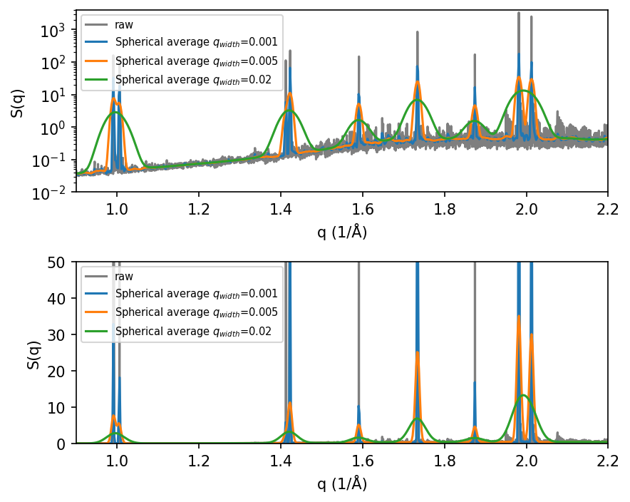
Note, that the position of the peaks in the static structure factor, \(S(q)\), obtained from MD agrees perfectly with the peaks obtained from the ideal tetragonal structure.
Convergence with respect to trajectory length#
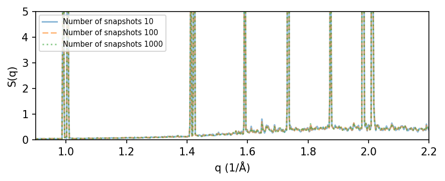
First, we analyze the static structure factor for a 8x8x8 tetragonal cell as a function of the simulation length (number of snapshots in the trajectory).
We analyze parts of the trajectory using 10, 100, and 1000 snapshots. The resulting S(q) looks quite converged already for 10-100 snapshots.
[7]:
%%time

q_width = 0.001
data_dict_nframes = dict()
for n_frames in [10, 100, 1000]:
    print('Running nframes', n_frames)

    # setup traj
    tag = f'tetra_size8_T450_nframes1000'
    dirname = f'md_runs/NVT_{tag}/'
    traj = Trajectory(dirname + 'movie.nc', trajectory_format='nc', frame_stop=n_frames)

    # generate all q-points in supercell
    q_points = get_spherical_qpoints(traj.cell, q_max=q_max)

    # compute Sq
    sample = compute_static_structure_factors(traj, q_points)
    sample_averaged = get_spherically_averaged_sample_smearing(sample, q_norms=q_linspace, q_width=q_width)
    data_dict_nframes[n_frames] = sample_averaged.q_norms, sample_averaged.Sq
Running nframes 10
INFO 2025-08-25 11:56:00: Length unit Angstrom and time unit ps inferred from trajectory.
INFO 2025-08-25 11:56:00: Trajectory file: md_runs/NVT_tetra_size8_T450_nframes1000/movie.nc
INFO 2025-08-25 11:56:00: Total number of particles: 5120
INFO 2025-08-25 11:56:00: Number of atom types: 1
INFO 2025-08-25 11:56:00: Number of atoms of type X: 5120
INFO 2025-08-25 11:56:00: Simulation cell (in Angstrom):
[[70.64849   0.        0.      ]
 [ 0.       70.64849   0.      ]
 [ 0.        0.       50.730995]]
INFO 2025-08-25 11:56:00: Number of q-points: 36893
Running nframes 100
INFO 2025-08-25 11:56:08: Length unit Angstrom and time unit ps inferred from trajectory.
INFO 2025-08-25 11:56:08: Trajectory file: md_runs/NVT_tetra_size8_T450_nframes1000/movie.nc
INFO 2025-08-25 11:56:08: Total number of particles: 5120
INFO 2025-08-25 11:56:08: Number of atom types: 1
INFO 2025-08-25 11:56:08: Number of atoms of type X: 5120
INFO 2025-08-25 11:56:08: Simulation cell (in Angstrom):
[[70.64849   0.        0.      ]
 [ 0.       70.64849   0.      ]
 [ 0.        0.       50.730995]]
INFO 2025-08-25 11:56:08: Number of q-points: 36893
Running nframes 1000
INFO 2025-08-25 11:57:04: Length unit Angstrom and time unit ps inferred from trajectory.
INFO 2025-08-25 11:57:04: Trajectory file: md_runs/NVT_tetra_size8_T450_nframes1000/movie.nc
INFO 2025-08-25 11:57:04: Total number of particles: 5120
INFO 2025-08-25 11:57:04: Number of atom types: 1
INFO 2025-08-25 11:57:04: Number of atoms of type X: 5120
INFO 2025-08-25 11:57:04: Simulation cell (in Angstrom):
[[70.64849   0.        0.      ]
 [ 0.       70.64849   0.      ]
 [ 0.        0.       50.730995]]
INFO 2025-08-25 11:57:04: Number of q-points: 36893
CPU times: user 1h 19min 24s, sys: 2.02 s, total: 1h 19min 26s
Wall time: 10min 3s
[8]:
# plot setup
fig = plt.figure(figsize=(6.0, 2.5), dpi=150)
ax1 = fig.add_subplot(111)
ylim = [2e-2, 5000]
alpha = 0.5

# plotting
linestyles = dict()
linestyles[10] = '-'
linestyles[100] = '--'
linestyles[1000] = ':'
for n_frames, (q, Sq) in data_dict_nframes.items():
    ax1.plot(q, Sq, ls=linestyles[n_frames], label=f'Number of snapshots {n_frames}', alpha=alpha)
ax1.set_xlabel('q (rad/Å)')
ax1.set_ylabel('S(q)')

ax1.set_xlim(xlim)
ax1.set_ylim(0, 5)
#ax1.set_yscale('log')
ax1.legend(loc=2, fontsize=7)

fig.tight_layout()
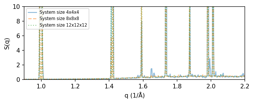
Convergence with respect to system size#
Next, we look at how S(q) converges with respect to system size in the MD simulation. For larger supercells the number of q-points becomes larger, meaning that the calculations will be slower. Running the last calculation, size=12, can take quite some time and running the full cell below can take a few minutes on a common workstation. To speed this up, we only use 100 frames from the trajectory (by setting frame_stop=100) and limit the number of q-points to 50,000 (by setting
max_points=50000)
[9]:
%%time

q_width = 0.001
size_vals = [4, 8, 12]
data_dict_sizes = dict()
for size in size_vals:
    print('Running size', size)

    # setup traj
    tag = f'tetra_size{size}_T450_nframes1000'
    dirname = f'md_runs/NVT_{tag}/'
    traj = Trajectory(dirname + 'movie.nc', trajectory_format='nc', frame_stop=100)

    # generate all q-points in supercell
    q_points = get_spherical_qpoints(traj.cell, q_max=q_max, max_points=50000)

    # compute Sq
    sample = compute_static_structure_factors(traj, q_points)
    sample_averaged = get_spherically_averaged_sample_smearing(sample, q_norms=q_linspace, q_width=q_width)
    data_dict_sizes[size] = sample_averaged.q_norms, sample_averaged.Sq
Running size 4
INFO 2025-08-25 12:06:04: Length unit Angstrom and time unit ps inferred from trajectory.
INFO 2025-08-25 12:06:04: Trajectory file: md_runs/NVT_tetra_size4_T450_nframes1000/movie.nc
INFO 2025-08-25 12:06:04: Total number of particles: 640
INFO 2025-08-25 12:06:04: Number of atom types: 1
INFO 2025-08-25 12:06:04: Number of atoms of type X: 640
INFO 2025-08-25 12:06:04: Simulation cell (in Angstrom):
[[35.324245  0.        0.      ]
 [ 0.       35.324245  0.      ]
 [ 0.        0.       25.365498]]
INFO 2025-08-25 12:06:04: Number of q-points: 4629
Running size 8
INFO 2025-08-25 12:06:06: Length unit Angstrom and time unit ps inferred from trajectory.
INFO 2025-08-25 12:06:06: Trajectory file: md_runs/NVT_tetra_size8_T450_nframes1000/movie.nc
INFO 2025-08-25 12:06:06: Total number of particles: 5120
INFO 2025-08-25 12:06:06: Number of atom types: 1
INFO 2025-08-25 12:06:06: Number of atoms of type X: 5120
INFO 2025-08-25 12:06:06: Simulation cell (in Angstrom):
[[70.64849   0.        0.      ]
 [ 0.       70.64849   0.      ]
 [ 0.        0.       50.730995]]
INFO 2025-08-25 12:06:06: Number of q-points: 36893
Running size 12
INFO 2025-08-25 12:07:02: Length unit Angstrom and time unit ps inferred from trajectory.
INFO 2025-08-25 12:07:02: Trajectory file: md_runs/NVT_tetra_size12_T450_nframes1000/movie.nc
INFO 2025-08-25 12:07:02: Total number of particles: 17280
INFO 2025-08-25 12:07:02: Number of atom types: 1
INFO 2025-08-25 12:07:02: Number of atoms of type X: 17280
INFO 2025-08-25 12:07:02: Simulation cell (in Angstrom):
[[105.97274   0.        0.     ]
 [  0.      105.97274   0.     ]
 [  0.        0.       76.09649]]
INFO 2025-08-25 12:07:02: Pruning q-points from the range 0.891 < |q| < 2.05
INFO 2025-08-25 12:07:02: Pruned from 124377 q-points to 50130
INFO 2025-08-25 12:07:02: Number of q-points: 50130
CPU times: user 39min 30s, sys: 1.68 s, total: 39min 32s
Wall time: 5min 6s
[10]:
# plot setup
fig = plt.figure(figsize=(6.0, 2.5), dpi=150)
ax1 = fig.add_subplot(111)
ylim = [2e-2, 5000]
alpha = 0.5

# plotting
linestyles = dict()
linestyles[4] = '-'
linestyles[8] = '--'
linestyles[12] = ':'
for size, (q, Sq) in data_dict_sizes.items():
    ax1.plot(q, Sq, ls=linestyles[size], label=f'System size {size}x{size}x{size}', alpha=alpha)
ax1.set_xlabel('q (rad/Å)')
ax1.set_ylabel('S(q)')

ax1.set_xlim(xlim)
ax1.set_ylim(0, 10)
#ax1.set_yscale('log')
ax1.legend(loc=2, fontsize=7)

fig.tight_layout()
Decomposing \(S(q)\) by atom types#
So far we have only considered the total \(S(q)\), but one can also decompose \(S(q)\) for the various atom types in the system and compute the partial structure factors \(S_{\alpha \beta}\).
\begin{equation*} S_{\alpha \beta}(\boldsymbol{q}) = \frac{1}{N} \left < \sum_{i \in \alpha} ^{N_\alpha} \sum_{j \in \beta}^{N_\beta} \exp{\left [ i\boldsymbol{q}\cdot (\boldsymbol{r}_i(t) - \boldsymbol{r}_j(t)) \right ]} \right >, \end{equation*}
where \(\alpha\) and \(\beta\) are different atom types, and \(N\) is the total number of atoms; see the dynasor documentation for more details on e.g. normalization.
Analyzing the partial structure factors can be useful in order to understand the origin of features and peaks in \(S(q)\), see e.g. this paper. Specifically, for CsPbI\(_3\) we know that it is displacements of the iodine atoms that give rise to the cubic to tetragonal phase transition, as we can clearly see below.
In order to compute the partial structure factors we need to specify atomic_indices in the Trajectory. By setting for example atomic_indices='read_from_trajectory' means the atomic types will be read directly from the trajectory, however this does not work for netcdf trajectories used in this tutorial. Instead we create a dict containing the atomic indices for each unique atom type using the input model.xyz file from which the MD simulations were started.
[11]:
q_width = 0.001
tag = f'tetra_size8_T450_nframes1000'
dirname = f'md_runs/NVT_{tag}/'

# read atomic indices
atoms_ideal = read(dirname + 'model.xyz')
atomic_indices = atoms_ideal.symbols.indices()
for atom_type, indices in atomic_indices.items():
    print(f'{atom_type}: num atoms {len(indices)}')

# setup traj
traj = Trajectory(dirname + 'movie.nc', trajectory_format='nc', atomic_indices=atomic_indices)

# generate all q-points in supercell
q_points = get_spherical_qpoints(traj.cell, q_max=q_max)

# compute Sq
sample = compute_static_structure_factors(traj, q_points)
sample_averaged = get_spherically_averaged_sample_smearing(sample, q_norms=q_linspace, q_width=q_width)
Cs: num atoms 1024
Pb: num atoms 1024
I: num atoms 3072
INFO 2025-08-25 12:11:11: Length unit Angstrom and time unit ps inferred from trajectory.
INFO 2025-08-25 12:11:11: Trajectory file: md_runs/NVT_tetra_size8_T450_nframes1000/movie.nc
INFO 2025-08-25 12:11:11: Total number of particles: 5120
INFO 2025-08-25 12:11:11: Number of atom types: 3
INFO 2025-08-25 12:11:11: Number of atoms of type Cs: 1024
INFO 2025-08-25 12:11:11: Number of atoms of type Pb: 1024
INFO 2025-08-25 12:11:11: Number of atoms of type I: 3072
INFO 2025-08-25 12:11:11: Simulation cell (in Angstrom):
[[70.64849   0.        0.      ]
 [ 0.       70.64849   0.      ]
 [ 0.        0.       50.730995]]
INFO 2025-08-25 12:11:11: Number of q-points: 36893
[12]:
# plot setup
fig, axes = plt.subplots(nrows=6, ncols=1, sharex=True, figsize=(6.0, 6.5), dpi=150)
ylim = [2e-2, 5000]
alpha = 0.5

# plotting
for ax, (atom_type1, atom_type2) in zip(axes, sample_averaged.pairs):
    key = f'Sq_{atom_type1}_{atom_type2}'
    ax.plot(sample_averaged.q_norms, sample_averaged[key], '-', label=f'{atom_type1} - {atom_type2}')
    ax.set_ylabel('S(q)')
    ax.set_xlim(xlim)
    ax.set_ylim(0, 35)
    ax.legend(loc=2)
    #ax.set_yscale('log')
ax.set_xlabel('q (rad/Å)')

fig.tight_layout()
fig.subplots_adjust(hspace=0)
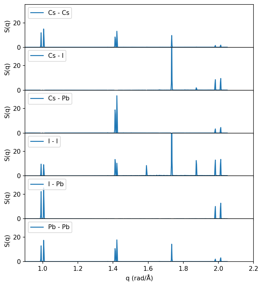
Note that the peaks around q=1.6 and q=1.85 (corresponding to the M-point as discussed above) only shows up in the I-I partial structure factor, as expected since the soft phonon mode at the M-point (corresponding to the transition from cubic to tetragonal) only involves I atoms.
Connecting to diffraction experiments#
The static structure factor, \(S(q)\), is closely connected to the measured intensity, \(I(q)\), in diffraction experiments, such as X-ray diffraction (XRD) or neutron diffraction. To obtain a one to one comparison one must weight the static structure factor with the corresponding form factors (cross-sections) for the relevant experiment, below we show how this can be done for X-rays.
[13]:
from dynasor.post_processing import XRayFormFactors
from dynasor.post_processing import get_weighted_sample

xlim = [0.7, 2.2]

# setup x-ray form factors
xrff = XRayFormFactors(sample_averaged.atom_types)

# weight sample with x-ray form factor
sample_weighted = get_weighted_sample(sample_averaged, xrff)

# convert q to theta
lam = 1.5406
n = 1
theta = np.arcsin(n * sample_averaged.q_norms * lam / 4 / np.pi) * 180 / np.pi

# plot both S(q) and I(q)
fig, (ax1, ax2) = plt.subplots(nrows=2, ncols=1, sharex=True, figsize=(6.0, 4.5), dpi=150)

ax1_v2 = ax1.twiny()
two_theta_ticks = np.arange(0, 40, 5)
ax1_v2.set_xticks([np.sin(two_theta / 2 / 180 * np.pi) / lam * 4 * np.pi for two_theta in two_theta_ticks])
ax1_v2.set_xticklabels(two_theta_ticks)
ax1_v2.set_xlim(xlim)
ax1_v2.set_xlabel(r'$2\theta$ (degrees)')

ax1.plot(sample_averaged.q_norms, sample_averaged.Sq, '-')
ax2.plot(sample_weighted.q_norms, sample_weighted.Sq, '-')

ax1.set_ylabel('S(q)')
ax1.set_xlim(xlim)
ax1.set_ylim(0, 50)
ax2.set_ylabel('I(q)')
ax2.set_xlim(xlim)
ax2.set_ylim(0, 150000)
ax2.set_xlabel('q (rad/Å)')

fig.align_ylabels()
fig.tight_layout()
fig.subplots_adjust(hspace=0)
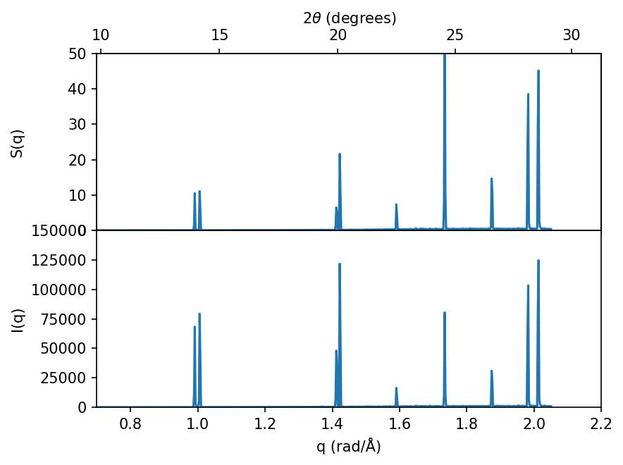
Note how all the peaks remain at the same positions, however the relative intensity (heights) between the peaks changes.
Observing the phase transition in \(S(q)\)#
Lastly, we show how the structure factor can be used to identify the phase transitions by running multiple simulations at various temperature and visualizing the results as a heatmap. Here, one can see how the peaks at the M-point (as discussed above) emerge at the phase transition temperature at around T=550 K.
See also Fig 4 in this paper for more details on this type of simulated diffraction patterns and how it can be used to track phase transitions